library(dplyr)
library(ggplot2)
library(brms)
library(tidybayes)
library(bayesplot)
library(gridExtra) # For grouping plots; optional
options(brms.backend = "cmdstanr")5 Flexible GLMs
Now that we can write brms models and read their output, we can brave more complicated models1. Let us consider some data from park visitors, gathered by UCLA. In their words:
The state wildlife biologists want to model how many fish are being caught by fishermen at a state park. Visitors are asked whether or not they have a camper, how many people were in the group, were there children in the group and how many fish were caught. Some visitors do not fish, but there is no data on whether a person fished or not. Some visitors who did fish did not catch any fish […]2
These data describe 250 groups of park visitors. For each group, we know how many fish they caught (count), how many total people were in the group (persons), how many of these were children (child), and whether the group brought a camper vehicle (camper).
fisher_df <- read.csv("https://paul-buerkner.github.io/data/fish.csv")
fisher_df <- fisher_df[, c("persons", "child", "camper", "count")]
names(fisher_df)[names(fisher_df) == "count"] <- "num_fish"
fisher_df <- fisher_df |>
  mutate(camper = as.factor(if_else(camper == 0, true = "no", false = "yes")))
summary(fisher_df)
Note that many visitor groups caught zero fishes (see Figure 5.1). These include zeroes from visitors that did not fish at all and zeroes from visitors that did fish but caught nothing.
Show histogram of fishes caught
ggplot(data = fisher_df, mapping = aes(x = num_fish)) +
  geom_histogram(binwidth = 2, color = "black", fill = "navyblue") +
  labs(
    title = "Many groups did not catch any fishes",
    x = "Fish caught",
    y = "Groups of visitors"
  ) +
  theme_bw()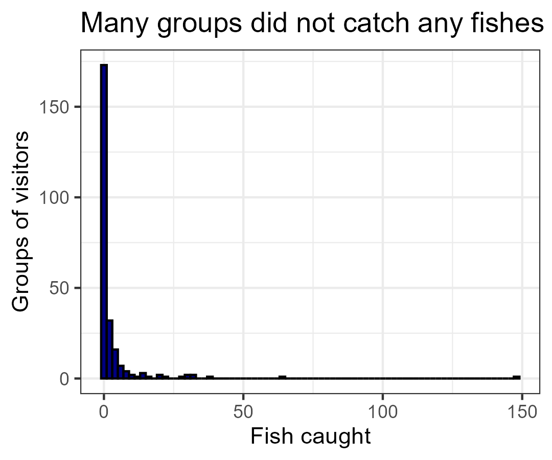
It is reasonable to think that larger groups were more likely to catch more fish. Also, groups with campers likely stayed longer at the park, which would give them more time to fish. And children dislike sitting in silence for long periods, so groups with more children may have fished less. These ideas suggest using a model that can associate the average number of caught fish to persons, child, and camper. We should also use a model that accounts for the fact that the number of fishes caught is a non-negative integer. A Poisson regression is a relatively simple model that can fulfil both of these requirements3.
An alternative to priors based on previous measurements is to use priors that discard implausible values but still allow wide ranges for all coefficients4. One common approach for this is to standardize all numerical dependent variables and assign them all a Normal distribution with mean zero and standard deviation 1. An equivalent approach is to rescale this distribution to match the scale of its corresponding variable.
The code to prepare these rescaled priors is below. Note that we have to use the alternative function prior_string(), which uses strings instead of formulas in its arguments. This allows us to compute the rescaled parameters without having to write them manually.
# Calculate SD for each predictor
sd_persons <- sd(fisher_df$persons)
sd_child <- sd(fisher_df$child)
prior_fisher1 <- prior_string(
    paste0("normal(0, ", 1 / sd_persons, ")"),
    class = "b",
    coef = "persons"
  ) +
  prior_string(
    paste0("normal(0, ", 1 / sd_child, ")"),
    class = "b",
    coef = "child"
  ) +
  prior(normal(0, 1), class = "b", coef = "camperyes") +
  prior(normal(0, 2.5), class = "Intercept")
Now we can fit our regression. The only novelty in the code below is the argument family, which controls the type of model we want to fit—in this case, a poisson().
fit_fisher1 <- brm(
  formula = num_fish ~ persons + child + camper,
  data = fisher_df,
  family = poisson(),
  prior = prior_fisher1,
  chains = 4,
  cores = 4,
  iter = 1000,
  warmup = 500
)
Once again, our ESS and R-hats are all acceptable:
summary(fit_fisher1) Family: poisson
Links: mu = log
Formula: num_fish ~ persons + child + camper
Data: fisher_df (Number of observations: 250)
Draws: 4 chains, each with iter = 1000; warmup = 500; thin = 1;
total post-warmup draws = 2000
Regression Coefficients:
Estimate Est.Error l-95% CI u-95% CI Rhat Bulk_ESS Tail_ESS
Intercept -1.97 0.15 -2.27 -1.67 1.00 1344 1117
persons 1.09 0.04 1.01 1.16 1.00 1410 989
child -1.68 0.08 -1.85 -1.53 1.00 1304 1298
camperyes 0.93 0.09 0.76 1.11 1.00 1490 1164
Draws were sampled using sample(hmc). For each parameter, Bulk_ESS
and Tail_ESS are effective sample size measures, and Rhat is the potential
scale reduction factor on split chains (at convergence, Rhat = 1).Before we examine the coefficients, we can check if our model can replicate the overall pattern of fish caught. The function pp_check() can paint many types of plots to illustrate how well our models fit the data. It asks us to define a model to evaluate and the type of evaluation we want. type = "hist" compares the histogram of the original data (shown as \(y\) in navy blue) to the histograms obtained from the random draws in our model (shown as \(y_{rep}\) in light blue). In this case, ndraws controls how many randomly chosen histograms to include in the plot.
pp_check(object = fit_fisher1, type = "hist", ndraws = 5, binwidth = 1) +
  coord_cartesian(xlim = c(0, 30)) +
  labs(
    title = "Poisson replicates data poorly",
    x = "Number of fish caught"
  ) +
  theme_minimal()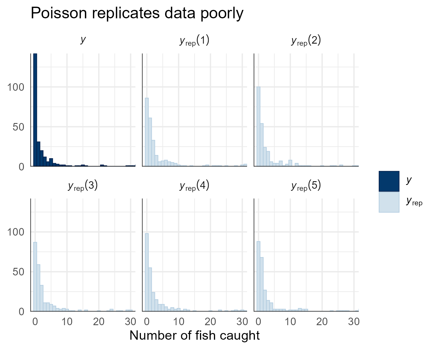
Figure 5.2 suggests that our model is predicting too many visitors with one, two, and three fishes and too few visitors with zero fishes. This suggests that, unfortunately, our current Poisson regression cannot account for these many zeroes, and in trying to do so it is distorting our inferences.
5.1 Handling excess zeroes
Fortunately, brms can expand our model so it directly estimates the proportion of groups that did not fish at all. This expanded model is called “zero-inflated Poisson regression” because it inflates (i.e., adds more) zeroes to the basic Poisson regression. For now, we presume that all groups had the same chance of going fishing. We do not change the default prior for the zero-inflation parameter, so the code to fit this zero-inflated regression is almost the same as before. The only change is that we now set the family to zero_inflated_poisson().
fit_fisher_zinf <- brm(
  formula = num_fish ~ persons + child + camper,
  data = fisher_df,
  family = zero_inflated_poisson(),
  prior = prior_fisher1, # Reuse prior from before
  chains = 4,
  cores = 4,
  iter = 1000,
  warmup = 500
)
Let’s see if our clever use of zero inflation paid off. First, it seems that our zero-inflated Poisson replicates well the overall pattern of fishes caught (see Figure 5.3).
pp_check(object = fit_fisher_zinf, type = "hist", ndraws = 5, binwidth = 1) +
  coord_cartesian(xlim = c(0, 30)) +
  labs(
    title = "Zero-inflated Poisson captures the data well",
    x = "Number of fish caught"
  ) +
    theme_minimal()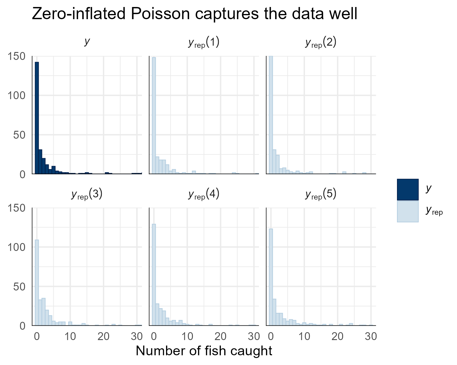
We can also inspect the proportion of visitors with zero fishes by calling pp_check() again. The code is similar to the one above, but we now use type = "stat" and add a custom function to compute the proportion of zeroes in a vector:
# Define a function that computes the proportion of zeroes
prop_zeros <- function(y) mean(y == 0)
pp_check(
  object = fit_fisher_zinf,
  type = "stat",
  stat = "prop_zeros",
  binwidth = 0.01
) +
  labs(
    title = "Zero-inflated Poisson captures zeroes well",
    x = "Proportion of visitor groups that caught zero fishes"
  ) +
    coord_cartesian(xlim = c(0.3, 0.8)) +
    theme_minimal() +
    theme(legend.position = "bottom")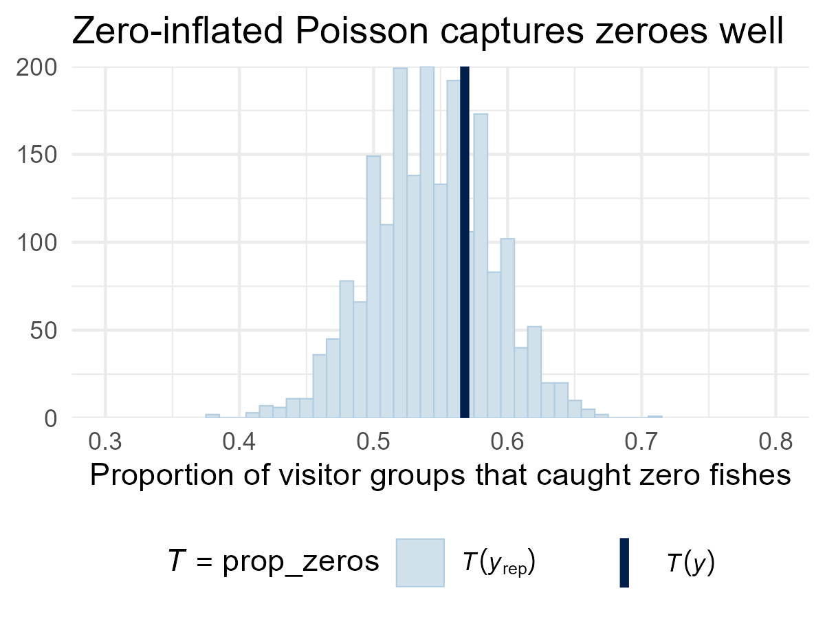
The figure above compares the observed proportion of zeroes (shown in navy blue) to the proportions predicted based on our model’s random draws (shown in light blue). As this histogram shows, our zero-inflated poisson accurately predicts the proportion of zeroes.
5.2 Interpreting Poisson
Now we can examine the coefficients from our more accurate zero-inflated Poisson regression. To flaunt the flexibility of brms’s output, we switch the width of the credibility intervals to 80%:
summary(fit_fisher_zinf, prob = 0.8) Family: zero_inflated_poisson
Links: mu = log
Formula: num_fish ~ persons + child + camper
Data: fisher_df (Number of observations: 250)
Draws: 4 chains, each with iter = 1000; warmup = 500; thin = 1;
total post-warmup draws = 2000
Regression Coefficients:
Estimate Est.Error l-80% CI u-80% CI Rhat Bulk_ESS Tail_ESS
Intercept -1.00 0.18 -1.23 -0.77 1.00 1425 1339
persons 0.87 0.04 0.81 0.93 1.00 1309 1286
child -1.36 0.09 -1.47 -1.24 1.00 1287 1222
camperyes 0.79 0.09 0.68 0.91 1.00 1677 1449
Further Distributional Parameters:
Estimate Est.Error l-80% CI u-80% CI Rhat Bulk_ESS Tail_ESS
zi 0.41 0.04 0.35 0.47 1.00 1582 1243
Draws were sampled using sample(hmc). For each parameter, Bulk_ESS
and Tail_ESS are effective sample size measures, and Rhat is the potential
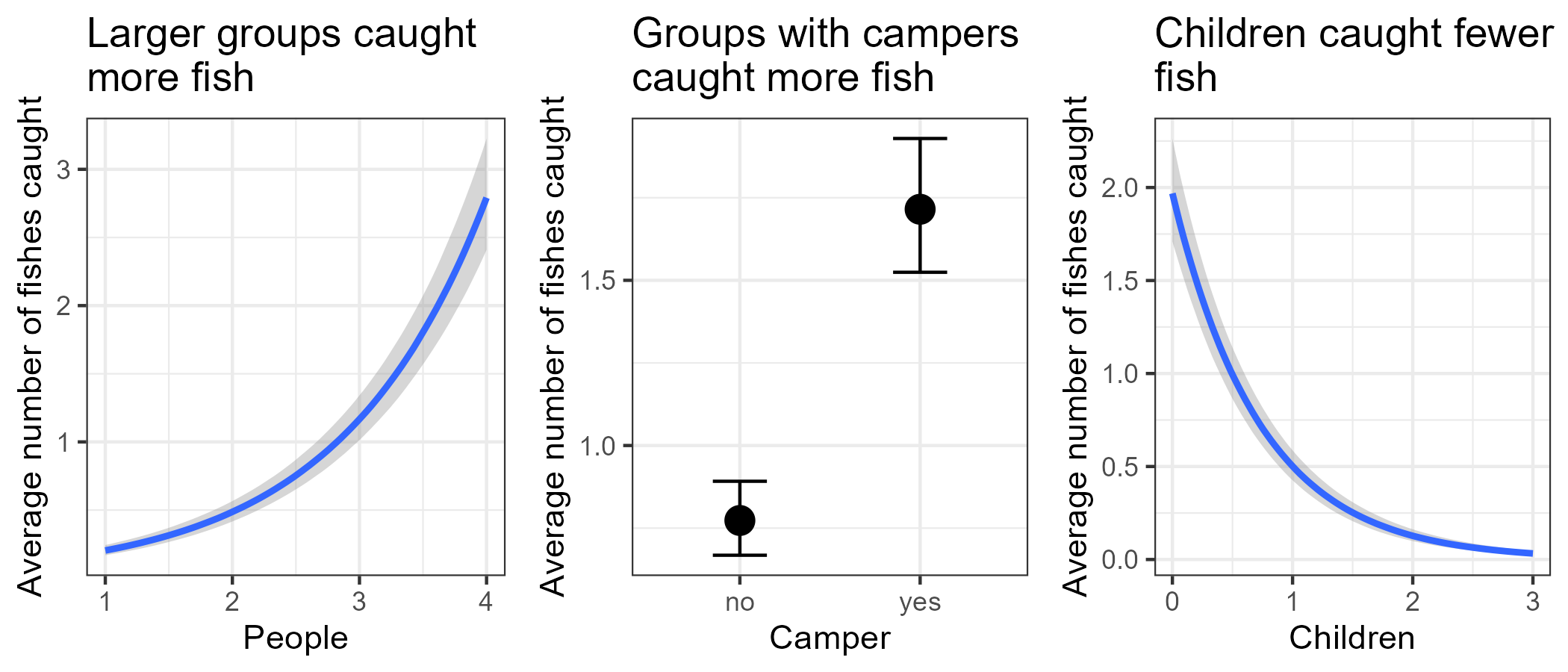
scale reduction factor on split chains (at convergence, Rhat = 1).For mathy reasons, the regression coefficients are in the natural logarithm scale, which complicates their interpretation. So, instead of deciphering the table, we can call conditional_effects() to plot the modeled associations between each variable and the average number of fish. The plots below show the medians and 80% credibility intervals of the posterior distributions of average fish at each value of the corresponding independent variable. When a variable is not shown in a plot, we are fixing its value at either its average (for continuous variables) or its reference category (for categorical variables).
We start by visualizing the association between average fishes caught and the number of people in a group:
conditional_effects(
    x = fit_fisher_zinf,
    method = "posterior_epred",
    effect = "persons",
    prob = 0.8 # For 80% credibility intervals
  )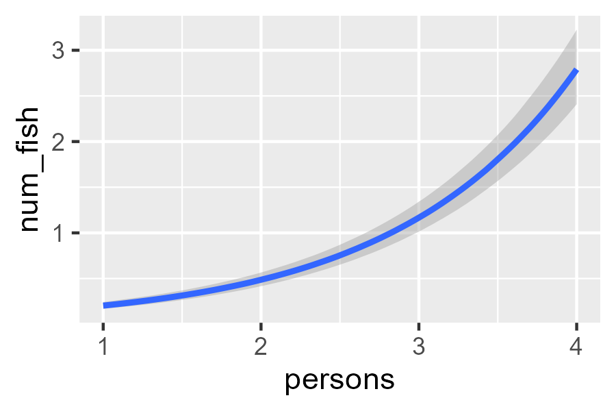
The main lesson from Figure 5.5 is that groups of visitors with more people caught more fish on average, but the difference was not big. With some effort, we can use ggplot to embelish this plot. We do the same for the associations of children and camper and show them together in Figure 5.6.
Grouped plots for conditional associations
# Number of people
person_assoc <- plot(
  conditional_effects(
    x = fit_fisher_zinf,
    method = "posterior_epred",
    effect = "persons",
    prob = 0.8
  ),
  plot = FALSE
)[[1]] +
  labs(
    title = "Larger groups caught\nmore fish",
    x = "People",
    y = "Average number of fishes caught"
  ) +
theme_bw()
# Children
child_assoc <- plot(
  conditional_effects(
    x = fit_fisher_zinf,
    method = "posterior_epred",
    effect = "child",
    prob = 0.8
  ),
  plot = FALSE
)[[1]] +
  labs(
    title = "Children caught fewer\nfish",
    x = "Children",
    y = "Average number of fishes caught"
  ) +
theme_bw()
# Camper
camper_assoc <- plot(
  conditional_effects(
    x = fit_fisher_zinf,
    method = "posterior_epred",
    effect = "camper",
    prob = 0.8
  ),
  plot = FALSE
)[[1]] +
  labs(
    title = "Groups with campers\ncaught more fish",
    x = "Camper",
    y = "Average number of fishes caught"
  ) +
theme_bw()
# Arrange these plots in a single row
grid.arrange(
  arrangeGrob(person_assoc, camper_assoc, child_assoc, ncol = 3),
  nrow = 1
)
Now let’s review the part of summary that refers to the zero-inflation parameter:
Further Distributional Parameters:
   Estimate Est.Error l-80% CI u-80% CI Rhat Bulk_ESS Tail_ESS
zi     0.41      0.05     0.35     0.47 1.00     1423     1407
In general, the parameter zi (short for “zero inflation”) represents the probability of an observation being an excess zero. In our model, we can interpret zi as the probability of not going fishing. With our current credibility criterion, this probability is estimated to be between 35% and 47%.