library(ggplot2)
library(brms)
library(tidybayes)
options(brms.backend = "cmdstanr")
data(penguins)
penguins$body_mass_kg <- penguins$body_mass / 10004 Tweaking regressions with brms
4.1 What do the numbers mean?
Let us return to our model for learning about the average penguin weight by species:
fit_weight1 <- brm(
    formula = body_mass_kg ~ species,
    data = penguins
)
We now know that Bayesian models use clever math to draw a bunch of random values to describe the parameters of interest. Figure 4.1 shows some colored histograms that represent the random draws—i.e., the posterior distributions—that brms got to describe each average penguin weight. The black dots are the estimated means of these histograms and the black bars around the black dots represent 95% credibility intervals of the average weights.
Posteriors of average weights
# Create a reference grid with one row per species
species_grid <- data.frame(species = c("Adelie", "Chinstrap", "Gentoo"))
# Extract posterior draws of the mean (epred = expected prediction)
posterior_means <- add_epred_draws(species_grid, fit_weight1)
ggplot(posterior_means, aes(x = .epred, y = species, fill = species)) +
  stat_histinterval(breaks = 20, point_interval = "mean_qi", .width = 0.95) +
  scale_x_continuous(breaks = seq(3.4, 5.6, by = 0.2)) +
  labs(
    title = "Chinstrap and Gentoo have similar average\nweights",
    x = "Average weight (kilograms)",
    y = "Species"
  ) +
  theme_bw() +
  theme(legend.position = "none")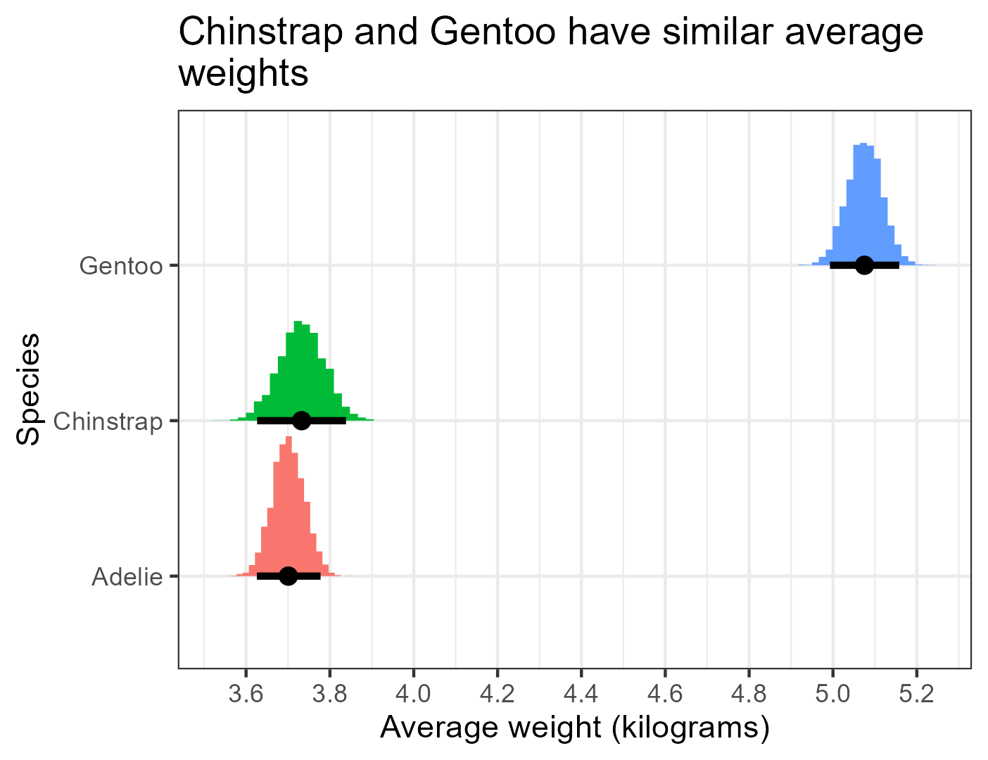
Now let us revisit the model summary we saw before:
Family: gaussian
  Links: mu = identity
Formula: body_mass_kg ~ species
   Data: penguins (Number of observations: 342)
  Draws: 4 chains, each with iter = 2000; warmup = 1000; thin = 1;
         total post-warmup draws = 4000

Regression Coefficients:
                 Estimate Est.Error l-95% CI u-95% CI Rhat Bulk_ESS Tail_ESS
Intercept            3.70      0.04     3.63     3.77 1.00     3794     2739
speciesChinstrap     0.03      0.07    -0.10     0.17 1.00     3977     2723
speciesGentoo        1.38      0.06     1.27     1.49 1.00     3844     3151

Further Distributional Parameters:
      Estimate Est.Error l-95% CI u-95% CI Rhat Bulk_ESS Tail_ESS
sigma     0.46      0.02     0.43     0.50 1.00     3943     2698

Draws were sampled using sample(hmc). For each parameter, Bulk_ESS
and Tail_ESS are effective sample size measures, and Rhat is the potential
scale reduction factor on split chains (at convergence, Rhat = 1).
These numerical summaries have enriched their meaning: they capture different parts of the histograms in Figure 4.1. Estimate shows their mean (painted as black dots), Est.Error shows their standard errors, and l-95% CI and u-95% CI show their 5% and 95% quantiles of the histograms (painted as black bars).
Other terms in the summary need elaboration, like chain, iter, warmup, Rhat, and Bulk_ESS and Tail_ESS. The formal definitions of these terms are very complicated, but an informal understanding is enough to fit almost all the models we need.
The random draws we get form a sequence or chain. Also, to get each random draw, brms goes through a computational process that it calls an iteration. The first few draws are usually too inaccurate to be useful, so we have to let the chain discard some warmup iterations.
Our penguin regression above used four chains, each of which had 2000 iterations, including warmup. Combining the post-warmup draws from all four chains gives us 4000 useful draws in total.
For complicated mathematical reasons, draws from a given chain tend to be related to each other, which makes them less informative than if they were independent. The effective sample size (ESS) measures the equivalent number of random draws we would have if our iterations were independent. A higher ESS means more reliable estimates. Bulk ESS measures the reliability of the center (or bulk) of our posterior distribution, e.g., the number we see in the Estimate column. Tail ESS measures the reliability of the tails of the posterior distribution, e.g., the numbers in columns l-95% CI and u-95% CI. So, having both a high Bulk ESS and high Tail ESS suggest that our histograms as a whole are reliable.
We want the effective sample size to be high enough to get stable estimates of uncertainty. In practice, this means that the ESS for all parameters should be above 400 in most models (Vehtari et al. 2021). Our penguin model above has way more ESS than this: the lowest Bulk ESS is 3794 (for the Intercept) and the lowest Tail ESS is 2698 (for the standard deviation sigma).
Finally, our chain is supposed to get draws for all the relevant values of the parameter of interest. However, with complicated models or difficult data, a chain can get stuck in a few specific values, depriving us of an accurate description of the posterior distribution. To check that we are getting all the relevant values, we should check that multiple chains converge to the same random values. In practice, we should use at least four chains when fitting any model.
R-hat (often styled \(\hat{R}\)) diagnoses convergence by comparing the variance of numbers within the chains to the variance across different chains. If the chains converged, these two variances should be roughly the same, so R-hat would equal 1. If the chains did not converge, the variances would differ and R-hat would be higher than 1.
In practice, an R-hat above 1.01 signals convergence problems and, therefore, unreliable results; an R-hat below 1.01 means that our chains converged well, so our results are reliable (Vehtari et al. 2021). Our penguin model shows that the R-hat for all parameters is practically 1. C’est magnifique!
4.2 The missing ingredient
So far, we have neglected the third ingredient of Bayesian cuisine: the prior distribution. A prior distribution describes what we know about the model parameters before, or prior to, analyzing our current data. This prior knowledge always exists and may come from previously published papers, related experiments, a formal theory, an informal familiarity, and sometimes from what we could call plain common sense. So, we can use the prior distribution to condense previous empirical work or to disregard implausible behaviors or relationships.
All Bayesian models have priors for all the parameters involved. brms has default priors that cover wide ranges of values. Especially so for regression parameters (excluding the intercept), which get assigned “flat” priors that, in rough terms, think that all real numbers are equally plausible. In our model above, for example, a flat prior for speciesGentoo says that, before seeing the data, we think that Gentoo penguins may be bigger than elephants or smaller than fleas.
Even a morsel of knowledge can lead to better priors than the defaults. Let’s pretend we have not yet fitted a regression. Wikipedia says that Adelie penguins weigh between 3.8 and 8.2 kg; that Chinstrap penguins weigh between 3.2 and 5.3 kg; and that Gentoo penguins weigh between 4.5 and 8.5 kg.
This knowledge suggests choosing our priors so that all average weights are between 4 and 8 kg; and so that most weights are within 1 or 2 kg of their averages. Note that Wikipedia was talking about the full ranges of weights, not just averages, so our priors are comparatively broad.
One way of defining our model’s priors is with the prior() function. The first, and unnamed, argument in prior() is the distribution1 we want to use. The second argument, class, is the type of parameter this distribution applies to. prior() accepts optional arguments lb and ub to implement hard limits on the parameter of interest. Use lb and ub only with parameters that have mathematical boundaries; standard deviations, for example, cannot be negative.
In this regression, we have to define three separate priors: one for the Intercept, one to apply to all other regression coefficients (nicknamed b in brms code), and one for the standard deviation of regression residuals (nicknamed sigma). The code to do this is shown below.
priors_weight1 <- prior(normal(6, 1), class = "Intercept") +
  prior(normal(0, 1), class = "b") +
  prior(normal(0, 2), class = "sigma", lb = 0)
In the code above, normal(0, 1) means “Normal distribution with mean equal to zero and standard deviation equal to 1”. I would like to name these parameters explicitly, but then the code would not run. The reason is that the code inside prior() is not for R but for Stan, so we have to conform to Stan’s syntax. And since writing things like mean = 0 inside distributions is illegal in Stan, we cannot write theme here either.
The Stan Functions Reference shows how to write all the parameters in any distribution it has; the Normal, for example, is here.
Now we refit our model with these new priors.
fit_weight2 <- brm(
    formula = body_mass_kg ~ species,
    data = penguins,
    prior = priors_weight1
)
summary(fit_weight2)
Family: gaussian
Links: mu = identity
Formula: body_mass_kg ~ species
Data: penguins (Number of observations: 342)
Draws: 4 chains, each with iter = 2000; warmup = 1000; thin = 1;
total post-warmup draws = 4000
Regression Coefficients:
Estimate Est.Error l-95% CI u-95% CI Rhat Bulk_ESS Tail_ESS
Intercept 3.70 0.04 3.63 3.78 1.00 3775 3195
speciesChinstrap 0.03 0.07 -0.11 0.16 1.00 3736 2989
speciesGentoo 1.37 0.06 1.26 1.48 1.00 3684 3021
Further Distributional Parameters:
Estimate Est.Error l-95% CI u-95% CI Rhat Bulk_ESS Tail_ESS
sigma 0.46 0.02 0.43 0.50 1.00 4175 3037
Draws were sampled using sample(hmc). For each parameter, Bulk_ESS
and Tail_ESS are effective sample size measures, and Rhat is the potential
scale reduction factor on split chains (at convergence, Rhat = 1).Our new results are very similar to the ones we had obtained using the default priors. In part because our data have enough evidence to avoid elephantine inferences. And in part because our Wikipedia-based priors overlapped with our data.
4.3 Turning knobs and pushing buttons
Our success in comparing penguins’ weight by species has made us more curious about these lovely amigos. Let us consider now, how much longer or shorter are the bills of male penguins compared to female penguins on average? Before we fit a regression, consider that bill length may be related to the size of the penguins, which in turn changes by sex and species. Figure 4.2 illustrates these associations.
Plot bill length by sex and species
ggplot(
  data = penguins,
  mapping = aes(x = body_mass_kg, y = bill_len, color = sex)
) +
  geom_point() +
  labs(
    title = "Males and heavier penguins have longer bills",
    x = "Body mass (kg)",
    y = "Bill length (mm)"
  ) +
  theme_bw() +
  facet_wrap(~species, nrow = 1) +
  theme(legend.position = "bottom")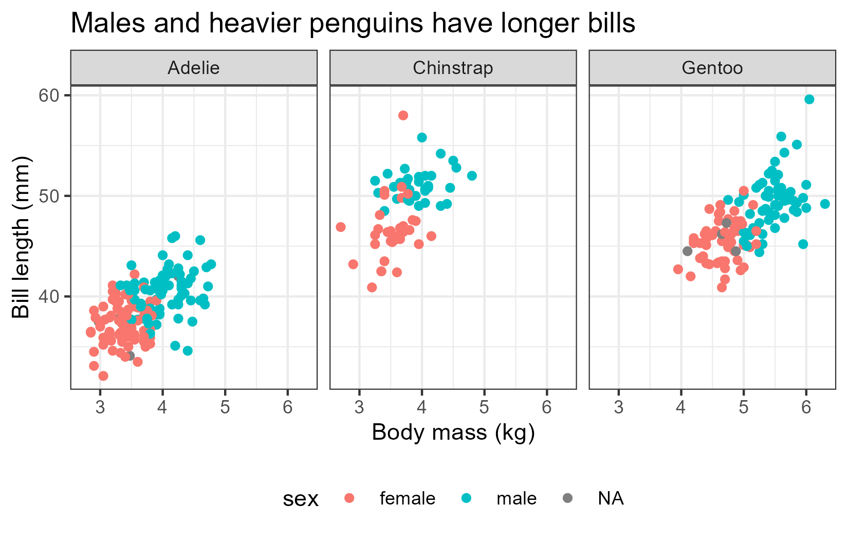
We could fit a regression with bill length (in milimiters) as the dependent variable, using sex as the independent variable and adding weight as a proxy for size. To make our model parameters easier to interpret, we will recenter weight (body_mass_kg) around its overall mean of 4.2 kg.
penguins$bm_kg_ctr <- penguins$body_mass_kg -
  mean(penguins$body_mass_kg, na.rm = TRUE)
To set our priors, note that the Intercept in brms represents the average value of the dependent variable when all independent variables are set to their average or to the reference category. With this in mind, we think that female Adelie penguins of average weight have a bill length of around 45 mm, and that bills of other types of penguins will be within 10 or 20 mm of this intercept. We also assign a more specific prior for the weight variable because we think it has a special association with bill length. To do this, we add a separate call of prior() and add the coef argument to specify the name of the variable.
priors_bill_len1 <- prior(normal(45, 10), class = "Intercept") +
  prior(normal(0, 10), class = "b") +
  prior(normal(0, 4), class = "b", coef = "bm_kg_ctr") +
  prior(normal(0, 20), class = "sigma", lb = 0)
We can fit our model more efficiently by changing the number of chains and iterations. By default, brms uses 4 chains, each with 2000 total iterations of which half are for warmup. Our model for bill length is relatively simple, so let’s try saving some computer time by using fewer iterations per chain. And let us be cool by having brms fit all the chains in parallel rather than one after the other.
fit_bill_len1 <- brm(
  formula = bill_len ~ sex + species + bm_kg_ctr,
  data = penguins,
  prior = priors_bill_len1,
  chains = 4,
  cores = 4, # for running chains in parallel
  iter = 800, # short for "iterations per chain" (this includes warmup)
  warmup = 400 # must be lower than iter
)
In the code above, the argument chains controls how many separate sequences of random values we will use. warmup controls how many random draws we will discard at the beginning. iter (short for iterations) controls the number of random draws per chain, which includes the warmup. cores controls the number of mini-brains in our computer that R will take. Each chain runs in one core, so we never need more cores than chains. In practice, ask for at most one core less than those available in your computer; the extra core will run everything else (e.g., internet browsers or Excel).
The regression summary below shows that the effective sample sizes for all parameters are well above the minimum threshold of 400, and all R-hats are equal to 1. And since R did not show any errors or concerning warnings, we can trust that our model ran appropriately.
summary(fit_bill_len1)Family: gaussian
Links: mu = identity
Formula: bill_len ~ sex + species + bm_kg_ctr
Data: penguins (Number of observations: 333)
Draws: 4 chains, each with iter = 800; warmup = 400; thin = 1;
total post-warmup draws = 1600
Regression Coefficients:
Estimate Est.Error l-95% CI u-95% CI Rhat Bulk_ESS Tail_ESS
Intercept 38.43 0.39 37.64 39.18 1.00 932 1011
sexmale 2.53 0.36 1.85 3.26 1.00 932 1004
speciesChinstrap 9.96 0.34 9.30 10.63 1.00 1633 1036
speciesGentoo 6.29 0.61 5.13 7.48 1.00 956 1134
bm_kg_ctr 1.73 0.39 0.95 2.49 1.00 897 1063
Further Distributional Parameters:
Estimate Est.Error l-95% CI u-95% CI Rhat Bulk_ESS Tail_ESS
sigma 2.27 0.09 2.10 2.45 1.00 1226 881
Draws were sampled using sample(hmc). For each parameter, Bulk_ESS
and Tail_ESS are effective sample size measures, and Rhat is the potential
scale reduction factor on split chains (at convergence, Rhat = 1).The coefficient for sexmale tells us that, if we took two penguins of the same species and average weight, we would expect the male penguin to have a bill that is between 1.85 and 3.26 mm longer on average than the female penguin.
A plot will help us visualize other regression results. First we define the coordinates that we want to see. expand.grid() can build a data frame with the coordinates we want to plot results for. We fill this function with the names and values of the variables we want to get. expand.grid() will then create all possible combinations of the values of these variables.
pred_grid <- expand.grid(
  sex = levels(penguins$sex),
  species = levels(penguins$species),
  bm_kg_ctr = seq(
    min(penguins$bm_kg_ctr, na.rm = TRUE),
    max(penguins$bm_kg_ctr, na.rm = TRUE),
    length.out = 50
  )
)
head(pred_grid)
sex species bm_kg_ctr
1 female Adelie -1.501754
2 male Adelie -1.501754
3 female Chinstrap -1.501754
4 male Chinstrap -1.501754
5 female Gentoo -1.501754
6 male Gentoo -1.501754Now we can combine the results from our model fit_bill_len1 with the values in pred_grid to paint regression values at these coordinates. add_epred_draws() uses the draws we got from brm() to compute many plausible averages of our dependent variable (bill length) many times. Finally, all these results are arranged in a format that is easy to plot with ggplot and other libraries. Luckily, the code to execute this rather involved process is blissfully simple:
posterior_lines <- add_epred_draws(
  newdata = pred_grid,
  object = fit_bill_len1
)
We can read the code above as “for each point of interest in pred_grid, we want ndraws draws from fit_bill_len1”. Omitting ndraws will ask add_epred_draws() to use all available draws in fit_bill_len1. Using more draws increases the precision of the plots we paint, but also the time it takes to draw them. 600 draws are usually precise and fast enough to plot and summarize results; we can use all the draws only when presenting the final results of an analysis.
Finally, we can combine ggplot with the tidybayes library to create a plot. stat_lineribbon() takes all the regression draws we saved in posterior_lines and, with some trickery, transforms them into a smooth plot. The thick lines represent the means and the shaded regions represent the credibility intervals of the average bill length at each weight.
# Save mean to return body mass to de-center body mass.
bm_kg_mean <- mean(penguins$body_mass_kg, na.rm = TRUE)
ggplot(
  data = posterior_lines,
  mapping = aes(
    x = bm_kg_ctr + bm_kg_mean,
    y = .epred,
    color = sex,
    fill = sex
  )
) +
  stat_lineribbon(
    point_interval = "mean_qi",
    .width = c(0.66, 0.9),
    alpha = 0.3
  ) +
  facet_wrap(~species) +
  labs(
    title = "Male penguins have slightly longer bills than females",
    x = "Body Mass (kg)",
    y = "Bill Length (mm)",
    color = "Sex",
    fill = "Sex"
  ) +
  theme_bw() +
  theme(legend.position = "bottom") +
  # OPTIONAL: Add observed data to plots
  geom_point(
    data = penguins,
    aes(x = bm_kg_ctr + bm_kg_mean, y = bill_len),
    alpha = 0.5,
    size = 1
  )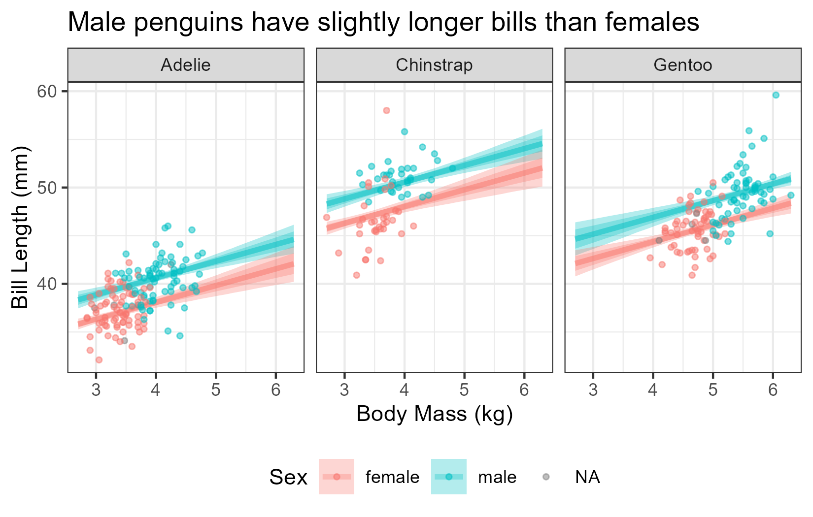
In stat_lineribbon(), point_interval controls the type of estimates that the plot will show, with "mean_qi" referring to using a mean and quantiles for the credibility intervals. .width controls the quantiles we use to delineate the credibility intervals. Using c(0.66, 0.9) uses quantiles for 66% and 90% credibility.
The list of available distributions and their parametrizations is available at https://mc-stan.org/docs/functions-reference/unbounded_continuous_distributions.html↩︎