2  A first regression in brms

library(ggplot2)
library(brms)
options(brms.backend = "cmdstanr")

brms allows us to add or remove parts of a model as needed, so our code is only as complicated as the model we want to fit. Simple code for simple models; fancy code for fancy models.

Imagine, for example, that we like penguins and we want to study their weight. R has some clean data about three types of chilly fellows: Adelie, Chinstrap, and Gentoo.

data(penguins)
penguins$body_mass_kg <- penguins$body_mass / 1000

To start, let us compare the weights of these three groups. The histogram below suggests that Gentoo penguins tend to be the heaviest, while Adelie and Chinstrap tend to have similar weights.

ggplot(penguins, mapping = aes(x = body_mass_kg)) +
    geom_histogram(binwidth = 0.2, color = "black", fill = "darkorange") +
    facet_wrap(~species, nrow = 3, ncol = 1) +
    labs(
    title = "Gentoo penguins are the heaviest",
    x = "Body mass (kilograms)",
    y = "Count"
    ) +
    theme_minimal()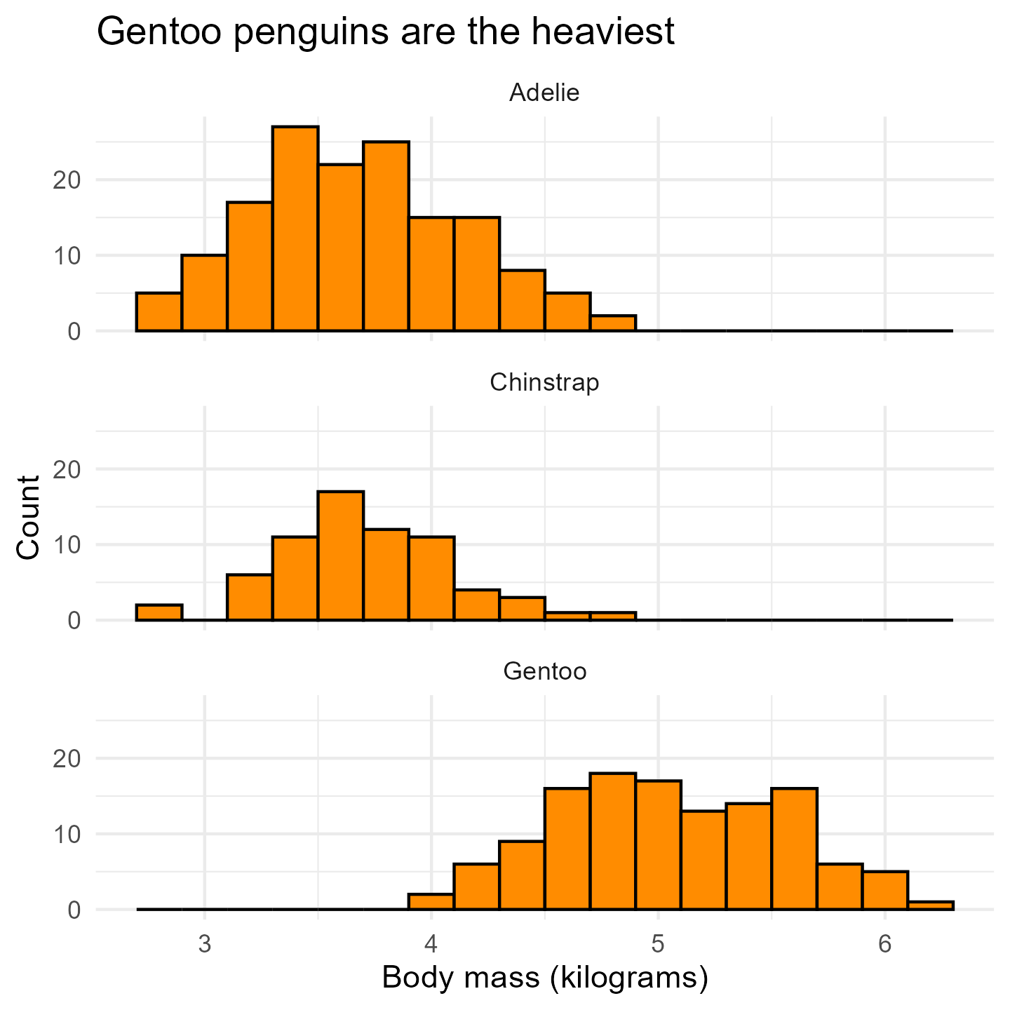

Figure 2.1: Three histograms show penguin weights

We can complement this histogram with estimates of the average weight of each group of penguins. A linear regression can give us these estimates along with their confidence intervals. We can fit this (and any other) regression in brms using the function brm() (short for “bayesian regression model”), which for our simple model requires only a formula to describe the regression function and the name of the data set that houses the corresponding variables.

The code below shows how to fit a linear regression with weight (in kilograms) as the dependent variable and species as the independent categorical variable with values “Adelie”, “Chinstrap”, and “Gentoo”. Run this code and ignore its lengthy output for now.

fit_peng1 <- brm(
    formula = body_mass_kg ~ species,
    data = penguins
)

The first time it sees a model, brm() compiles the code, i.e., it uses the C++ toolchain to translate the code into efficient machinespeak. brm() does not need to recompile unless we change something, so rerunning this same regression will be much faster (try it!). Think of brm() as a virtual chef that can cook many things but has to prepare the kitchen after we tell it what we want.

Now we can ask the model what it thinks the average weights are. Understanding where these values above come from requires a taste of Bayesian statistics that we will savour soon. For now, though, we can summarize our results as follows, focusing on the table of regression coefficients.

summary(fit_peng1)

Family: gaussian
  Links: mu = identity
Formula: body_mass_kg ~ species
   Data: penguins (Number of observations: 342)
  Draws: 4 chains, each with iter = 2000; warmup = 1000; thin = 1;
         total post-warmup draws = 4000

Regression Coefficients:
                 Estimate Est.Error l-95% CI u-95% CI Rhat Bulk_ESS Tail_ESS
Intercept            3.70      0.04     3.63     3.77 1.00     3794     2739
speciesChinstrap     0.03      0.07    -0.10     0.17 1.00     3977     2723
speciesGentoo        1.38      0.06     1.27     1.49 1.00     3844     3151

Further Distributional Parameters:
      Estimate Est.Error l-95% CI u-95% CI Rhat Bulk_ESS Tail_ESS
sigma     0.46      0.02     0.43     0.50 1.00     3943     2698

Draws were sampled using sample(hmc). For each parameter, Bulk_ESS
and Tail_ESS are effective sample size measures, and Rhat is the potential
scale reduction factor on split chains (at convergence, Rhat = 1).

The Intercept represents the average weight of our Adelie penguins, while speciesChinstrap and speciesGentoo represent the differences of the averages of Chinstrap and Gentoo relative to Adelie. The column Estimate represents a clever guess of the values of the coefficients; Est.Error represents the margin of error of this guess; and l-95% CI and u-95% CI represent the limits of the credibility interval (similar to a confidence interval), a range for the most plausible values of the coefficient.

Based on these results, we estimate that both Adelie and Chinstrap weight around 3.7 kilograms on average, while Gentoo penguins weight around 5.08 kilograms on average. We also estimate that the standard deviation of the weight of all penguin groups, sigma, is 0.46, which means that most penguins’ weights lie within 0.92 kilograms of their group average.

The summaries we just saw suffice to understand the elementary aspects of many regression models. But the power and versatility of brms will be easier to wield if we devote a little time to learning the “bayesics” of Bayesian statistics and computation. We just learned how to turn on the oven. A bit more effort and we can learn to control the heat.