1 The Basics of Stata
1.1 The Stata Environment
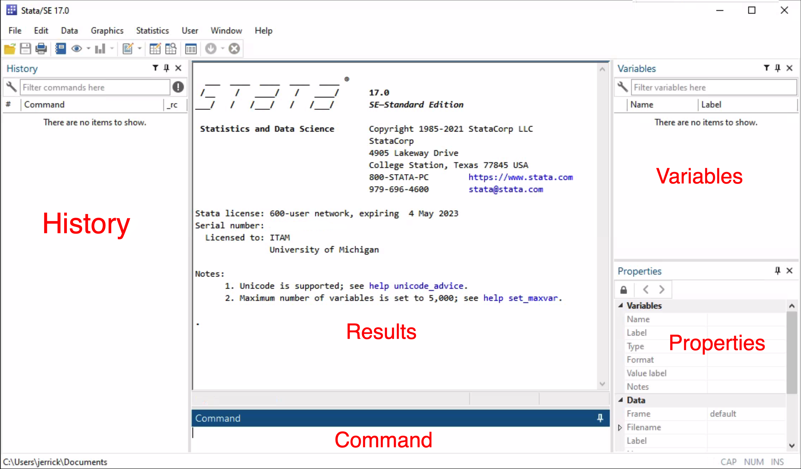
When a user first opens Stata, there are five panes that will appear in the main window:
- The Results Pane
- All commands which are run are echoed out here, as well as any output they produce. Not all commands produce output though most do (e.g. obtaining summaries of the data or running a statistical procedure). Items that appear in the results pane in blue are clickable.
- The Command Pane
- This pane is where users can interactively type Stata commands and submit them to Stata for processing. Everything that one can do in Stata is based on a set of Stata commands. Stata commands are case sensitive. All Stata commands and options are in lower case. When variables are used in any command, the variable names are also case sensitive.
- The Variables Pane
- This pane displays all of the variables in the data set that is currently open in Stata, and users can click on variable names in this pane to carry the variables over into Stata commands in the Command pane. Note that Stata allows only one data-set to be open in a session.
- The History Pane
- Stata will keep a running record of all Stata commands that have been submitted in the current session in this pane. Users can simply click on previous commands in this pane to recall them in the Command pane.
- The Properties Pane
- This pane allows variable properties and data-set properties to be managed. Variable names, labels, value labels, display formats, and storage types can be viewed and modified here.
Each of these five panes will be nested within the main Stata session, which contains menus and tool bars. There are additional windows that users can access from the Window menu, which include the Graph window (which will open when graphs have been created), the Viewer window (which is primarily used for help features and Stata news), the Data Editor window (for use when viewing data sets), and the Do-file Editor window (for use when writing .do files).
In the lower left-hand corner of the main Stata window (below the panes), there will be a directory displayed. This is known as the working directory, and is where Stata will look to find data files and other associated Stata files unless the user specifies another directory. We will cover examples of changing the working directory.
1.1.1 Alternate Layout
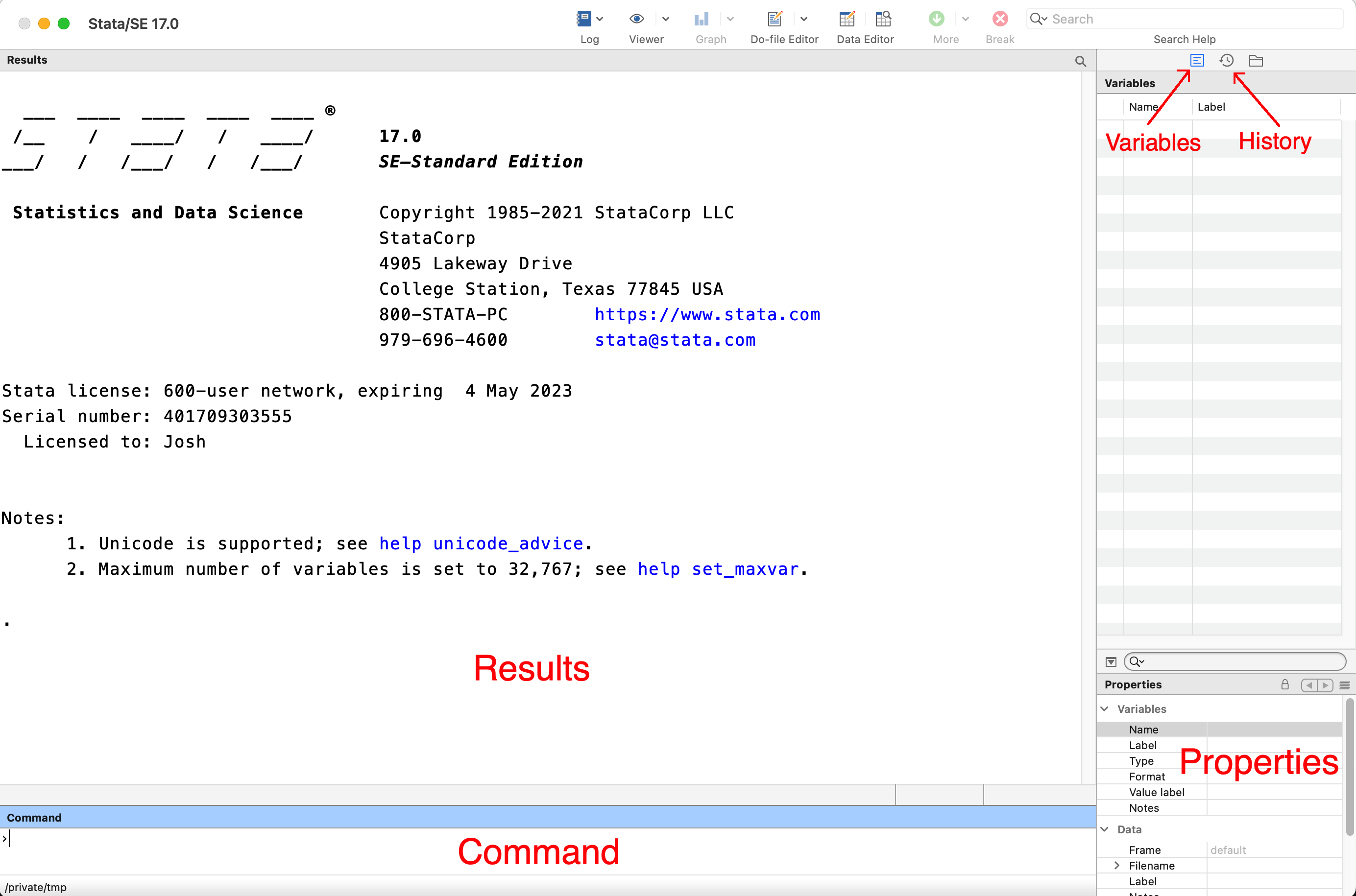
An alternate layout (found in View -> Layout) places the History and Variables pane in tabs on the right hand side instead.
(Note that this screenshot is taken on a Mac, as opposed to the original screenshot on Windows, just for comparison.)
1.2 One Data
One functionality where Stata differs than most other statistical or data analysis software is that Stata can only work with a single data set at a time.
Any command you run knows to operate on the data set you have open. For example, there is a command summarize which provides summary information about variables. The command is simply summarize, there is no need to direct it towards a specific data set.
If you have multiple data sets you need to work with, you can either
1.3 Give Stata a command
Let’s try running a Stata command. In the command pane, type (or copy and paste) the following:
versionThe following should appear in the Results pane:
. version
version 18.5
The first line proceeded by the . indicates the command that was written, version, and the rest is the output. Here, I am running Stata version 18.5 (your version may vary).
In this document, if you see a single command without a period, it indicates something that was not run - either it’s not designed to be run (it’s fake code designed to illustrate a point), or more likely, the output is not interesting or unnecessary. If you instead see a Results output where the first line is the command prefaced by the ., that was run in Stata and only the Results are included since they include the command. The command can still be run, but should be run without the .1.
1.3.1 Saving Results
Any output that appears in the Results pane (including the echoed commands and any errors) can be copied and pasted into another location, such as Word. In addition, if you highlight text and right-click, you also have the options:
- “Copy table”: Useful for exporting to Excel. This can be tempermental; if the selected table is less “regular”, this may not produce the best results. It is most useful for text which comes naturally as a table rather than results which are forced into a table for display purposes.
- “Copy table as HTML”: You can paste this into a plaintext editor (Notepad.exe or TextEdit, not Word) and save it as a *.qmd to produce a webpage. If you paste this into Excel you get a slightly different table than the layout for “Copy table” which may be more useful.
- “Copy as picture”: Does exactly what it says - equivalent to taking a screenshot. Very handy!
There are a few commands that can be useful for saving results which we will not cover in this workshop, if you are interested, you can look into the help for them.
log: Saves a file consisting of everything printed to the Results pane.putexcel: Adds to a spreadsheet specific strings or output.dtable: A very complex command that can create complete tables. Take a look at this blog post on the Stata blog for more ideas of how it can be used.outreg2: A user-written command to output the results of a model (e.g. regression) in a clean format.
1.4 Updating
If you have administrative access on your computer (e.g. if it is your personal machine, or your IT department has given you the ability), you can update Stata freely. Major point upgrades such as 18.0 require purchase and re-installation, but minor upgrades (such as the 16.1 and 16.2 updates) as well as minor internal updates are usually free.
To check for updates, you can run
update queryIf any updates are available (regardless of whether you ran a query first), you can obtain all updates with
update allIf you do not have administrative access on your computer, you’ll need to reach out to your IT administrators to update.
1.5 Installing user-written commands
In addition to built in commands, Stata supports user-written programs, know as “ado-files”2. Once installed, these user-written programs operate identically to any built-in command, with the caveat that they may not be quite as polished or complete since they’re volunteer written. Documentation is rarely up to Stata standards and often relegates details to a manuscript.
We won’t be covering any ado-files in these notes, but if you wanted to install a program named newcommand:
ssc install newcommandYou can remove a program with
ssc uninstall newcommandFinally, to see a list of all user-written programs you have installed, used
adoUpdating Stata will not update any ado-files, instead you can run
adoupdateto list all available updates and
adoupdate, updateto perform all updates.
1.6 Do-files
We saw that commands can be typed interactively, one command at a time, and the results immediately observed. From this, the output can be copied/exported/printed, or the results can be saved. However, a better paradigm would save all the commands run separately so that the analysis is reproducible.
For this purpose, Stata has Do-files (named because they are saved with the .do extension, such as analysis.do) which are scripts containing only commands and comments. We can then run any subset of the commands (including the entire file), re-running parts or all of the analysis. Additionally you can easily save and/or share this command, allowing yourself or a colleague to re-run the analysis.
There are several ways to start a new Do-file.
- File -> New -> Do-file
- Click the “Do-file Editor” button in the main window
- You can enter the command:
doedit- If you select some commands in the History pane, you can right click and choose “Send select to Do-file Editor”.
For the last option there, note that performing that twice will create two separate Do-files instead of appending the commands. Instead, you can copy and paste from the History pane to add to an existing Do-file.
Let’s manually add some commands to a Do-file to see how to execute the commands. In a Do-file editor, enter the following
sysuse auto, clear
summarize price
tabulate foreign
Once the lines are in the editor, highlight the commands (you do not need to highlight the entire line, you merely need to ensure your selection includes part of every line you want run) and press the “Execute/Do” (on Windows) or “Do” (on Mac) button. You should see the following appear in your Results pane.
. sysuse auto, clear
(1978 automobile data)

. summarize price

    Variable |        Obs        Mean    Std. dev.       Min        Max
-------------+---------------------------------------------------------
       price |         74    6165.257    2949.496       3291      15906

. tabulate foreign

 Car origin |      Freq.     Percent        Cum.
------------+-----------------------------------
   Domestic |         52       70.27       70.27
    Foreign |         22       29.73      100.00
------------+-----------------------------------
      Total |         74      100.00
We will cover in later sections what each of these commands does (sysuse, summarize, and tabulate).
1.6.2 Version control
When writing a Do-file, you generally are creating it while using a single version of Stata. If a new version of Stata were released, its possible that your code may operate differently with the new version. If you add
version 14.2to the beginning of your Do-file, Stata will execute the commands as if it were still running version 14.2, even if you’ve updated to Stata 18. This works all the way back to Stata 2. (Obviously, this will not work if you try to run as Stata 18 when you only have Stata 14 installed.)
Note that this version is the same command as the version we’ve been discussing before. It operates in this special fashion only when included at the top of a Do-file.
Best practices is to always include a version ##.# line at the top of each Do-file, but if its code that will continue to see use, you should test it with the newer releases and update the code as necessary!
1.7 Exercise 0
Get familiar with the Stata interface. If you’ve been following along, you may have already done all these!
- If you haven’t already, open Stata. (You should be able to do this by clicking on the “Start” menu in the bottom left of the screen, then typing “Stata”.)
- The use of each pane will become much clearer when we start opening data in the next section, but take a look at each.
- Give Stata a command:
query memory. This lists some settings related to memory usage in Stata, for example,maxvaris the maximum number of variables in a model;matsizeis the largest number of predictors allowed in a model. - Open a Do file. Place a
versioncommand at the top of the file corresponding to the version on your computer. Place thequery memorycommand from the last step in the Do file. - Be sure you know how to run these commands from the Do file.
- Comment out the
query memorycommand; we won’t need it anymore.
1.8 Basic command syntax
Most Stata commands which operate on variables (as opposed to system commands such as version, update, query, etc.) follow the same general format. Recognizing this format will make it easier to understand new commands to which you are introduced.
The basic syntax is
command <variable(s)>, <options>The command can take on more than one word; e.g. to create a scatter plot, the command is graph twoway scatter.
Depending on the command, the list of variables can contain 0 variables, 1 variable, or many variables separated by spaces. Whether the order of variables matters depends on the specific command.
Above, in the do-file, we ran three lines of code. The first, sysuse auto, is a system command that we’ll discuss later.
The second and third lines, summarize price mpg and tabulate foreign, follow the basic syntax - “summarize” and “tabulate” are the commands. “summarize” is operating on two variables, “price” and “mpg”; the order in which the variables appear in the command controls the order in which they appear in the table. “tabulate” is operating on a single variable, creating a one-way table; putting a second variable transforms it into a two-way table.
The options are not required (none of the above commands have options), but if they are given, they too are separated by spaces. There are some options that are consistent across a number of commands, and some options are specific to commands.
1.9 Stata Help
Stata has, hands down, the best built-in help files of any of the “Big 4” statistical software.3 Stata’s help should be your first stop for any of the following:
- Understanding the syntax of a command
- Exploring the options available for a given command
- Looking at examples of the command in use
- Understanding the theoretical statistics behind the command.
Help can be accessed by calling help <command>, such as
help summarizeEach help page has numerous features, I will merely point out a few here.
- The “Title” section contains a link (in blue) to a PDF which contains the Manual, which has more detail and examples than the help file alone.
- The syntax section shows the basic syntax. Any part written in square brackets (
[...]) are optional. - The examples in the help are great but basic; the PDF help (see #1) usually has more detailed examples.
- We will discuss the “Stored results” in the [Programming][programming] section.
help can also be used to search for the appropriate command. For example, if you wanted help merging some data together (which we will cover [later][merging files]), you might try running
help mergingmerging is not a valid Stata command, so instead Stata performs a search of the help files. This search is often not great. I would recommend searching online for the appropriate command to use (just search “Stata” and what you are trying to do), then using the built-in help for details on using the command.
Finally, help help works and brings up some more information on the help command.
1.9.1 Short commands
You’ll frequently see commands with partial underlining; for example summarize has the “su” underlined. Only the underlined part needs to be given for Stata to understand the command; e.g. the following are all equivalent:
summarize
summ
su
This is often true for options as well; detail (to report far more summary details) has the “d” underlined. So these are equivalent:
summarize, detail
su, detail
summarize, d
su, d
The short commands are very useful for quickly writing commands, but not so great at reading them. If you came across someone else’s Stata Do-file and saw su, d, you might have trouble figuring that out unless you already knew that short command. Thankfully, the short commands can be used with help, so help su will bring up the full summarize documentation.
1.10 Working directory
We mentioned earlier the notion of a “working directory”, the current one you can see in the bottom left of the Stata window. You can think of a working directory as an open folder inside Windows Explorer (or Finder if you’re on a Mac). You can easily access any file within that folder without any additional trouble. You can access files in other folders (directories), but it requires moving to that folder.
In the same sense, when referring to files, any file in the working directory can be referred to buy its name. For example, to open a file (we’ll go into detail about doing this later) named “mydata.dta” which is in your current working directory, you need only enter
use mydata.dta(Technically you could just run use mydata as Stata will search for a file with the appropriate “.dta” extension automatically.)
If you were in a different working directory, you need to specify the full path to the file:
use C:\Documents\Stata\Project\mydata.dtaSimilarly, when saving files, the working directory is the default choice.
If your file path has any spaces, you must wrap it in quotations:
use "C:\Documents\Stata\My Project\mydata.dta"The working directory can be viewed with the pwd command (Print Working Directory)
. pwd
C:\Documents
You can change the working directory by passing a path to cd (Change Directory):
cd C:\Documents\Stata\ProjectAlternatively and perhaps more easily, you can change the working directory by the menus, choosing “Files -> Change working directory”. After selecting the appropriate directory, the full cd command will be printed in the Results, so you can save it in a Do-file for later use.
1.10.1 File paths
There are some distinctions between Windows and Mac in regards to file paths, the most blatant that Windows uses forward slash (\\) whereas Mac uses back slashes (\/). You can see full details of this by running help filename.
Stata can handle commands that are prefaced by
.(with a space between the period and comand) so you can copy/paste the. versionand run it as is. However, don’t get used to that habit! The correct command is justversion.↩︎As we’ll see in a bit, you can save Stata commands in a “do-file”. While I’ve never seen an official definition, I tend to think of “ado” as “automatic do”.↩︎
I consider the “Big 4” as Stata, SAS, SPSS, and R. SPSS has terrible help; SAS’s is good but dense and difficult to navigate if you don’t already know what you’re looking for; R’s is very hit-or-miss depending on who wrote it.↩︎
1.6.1 Comments
Comments are information in a Do-file which Stata will ignore. They can be used to stop a command from running without deleting it, or more usefully, to add information about the code which may be useful for others (or yourself in the future) to understand how some code works or to justify why you made certain choices. In general, comments can also help readability. There are three different ways to enter comments (and one additional special way).
First, to comment out an entire line, precede it by
*:Second, you can add a comment to the end of a line with
//There must be a space before the
//if it comes after a command:Thirdly, you can comment out a section by wrapping it in
/\*and\*/Note that when a command wraps to more than one line in the Results pane (either due to a manual line break like this or a command that’s too wide for the Results pane), the prefix changes from
.to>to indicate that its all one command.Finally, there’s the special comment,
///. Stata commands must be on a single line. However, complicated commands may get very long, such that its hard to read them on a single line. Using///instead of//allows wrapping onto the next line.As with
//, there needs to be a space before the///.Only the
*works on interactive commands entered in the Command pane. All four versions work in Do-files.