2 Working with Data Sets
2.1 Built-in data
Before we turn to using your own data, it is useful to know that Stata comes with a collection of sample data sets which you can use to try the Stata commands. Additionally, most (if not all) of the examples in Stata help will use these data sets.
To see a list of the built-in data sets, use
. sysuse dir
  auto.dta        census.dta      network1.dta    surface.dta
  auto16.dta      citytemp.dta    network1a.dta   tsline1.dta
  auto2.dta       citytemp4.dta   nlsw88.dta      tsline2.dta
  autornd.dta     educ99gdp.dta   nlswide1.dta    uslifeexp.dta
  bplong.dta      gnp96.dta       pop2000.dta     uslifeexp2.dta
  bpwide.dta      lifeexp.dta     sandstone.dta   voter.dta
  cancer.dta      mycensus9.dta   sp500.dta       xtline1.dta
and use sysuse again to load data, for example the auto data which contains characteristics of various cars from a 1978 Consumer’s Report magazine.
. sysuse auto
(1978 automobile data)
If you make any modifications to your data, Stata will try and protect you by refusing to load a new data set which would dispose of your changes. If you are willing to dispose of your changes, you can either manually do it by calling
clearor passing it as an option to sysuse,
. sysuse auto, clear
(1978 automobile data)
2.1.1 Stata Website Data
In addition to the data sets distributed with Stata, Stata also makes available a large collection of data sets on their website which can be accessed with the webuse command. These data sets are used as examples in the Manual and can be seen listed as http://www.stata-press.com/data/r18/.
webuse hiwaywebuse supports the clear option as well.
The exercises in this workshop will be using mostly built-in data sets as it makes distribution easy!
2.2 Opening data
You may have guessed from the sysuse and webuse commands that the command to load local data is use:
use <filename>As discussed in the working directory section, Stata can see only files in its working directory, so only the name of the file needs to be passed. If the file exists in a different directory, you will need to give the full (or relative path). For example, if your working directory is “C:\Documents\Stata” and the file you are looking for, “mydata”, is in the “Project” subfolder, you could open it with any of the following:
use C:\Documents\Stata\Project\mydata
use Project\mydata
cd Project
use mydata
Note that if the path (or file name) contains any spaces, you need to wrap the entire thing in quotes:
use "C:\Documents\Stata\My Project\My Data"It is never wrong to use quotes (just not always required), so perhaps that’s a safer option.
If the location of your file is much different than your working directory, it can be quicker just to use the menu “File -> Open” and use the file open dialog box instead. As with all commands, the use command will be echoed in the Results after using the dialog box, allowing you to add it to a Do-file.
As with sysuse and webuse, the clear option discards the existing data regardless of unsaved changes.
2.2.1 Loading subsets of the data
You can load only a subset of the data into the program at a time. Generally I would recommend loading the full data and then discarding the extraneous information. However, if your data is very large, it might be handy to only load in some of it rather than the entire thing. As this is a lesser-used option we won’t go into too much detail, but as an example, if I wanted to load only the variables named “bp”, “heartrate” and “date” from the data set “patientdata”, restricted to male patients, I might use something like
use bp heartrate date if gender == "male" using patientdataHere, using and if are subcommands, which we will see used more as the day goes on.
The statement gender == "male" is a conditional statement which only loads male patients. We’ll discuss later about conditional statements.
Alternatively, if you have a very large data set, you can load in a small chunk of it.
use patientdata in 1/100This loads just the first 100 rows (a/b is a “numlist” counting from “a” to “b” by integers).
For further details, see help use, specifically the manual which has the full documentation.
2.3 Editing data manually
We will discuss in Data Manipulation how to edit your data on a larger scale and in an automated fashion, but Stata does support modifying a spreadsheet of your data similar to Excel. At the top of the main window, you’ll see two buttons, “Data Editor” and “Data Browser”. These open the same new Data window, the only difference is that Stata is protecting you from yourself and if you open the “Data Browser” (or switch to it in the Data window), you cannot modify the data.
Once in the Data window, you can select cells and edit them as desired. Note that whenever you make a modification in the Data Editor, there is a corresponding command produced which actually performs the modification.
. replace age = 27 in 11
(1 real change made)
2.3.1 Colors as variable type
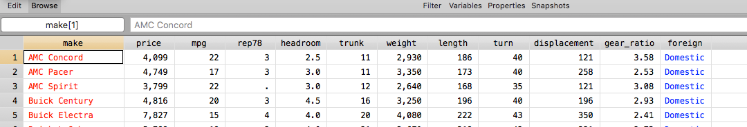
When viewing the data, the color of each column’s text provides information about the type of variable. We’ll go into more details later what these types mean. Below, for the auto data, you can see the make variable is red, indicating a string, the foreign variable is blue indicating a variable with an attached value label and the remainder of the variables are black for numeric.
2.4 Saving data
Saving data is done with the save command. There are two variations of running.
save, replaceIn this first variation, by not giving a file name and passing the replace option, Stata will overwrite whichever file you loaded with use. (It will error if you loaded a file via sysuse or webuse.)
The second variation takes a file name:
save newfile
save newfile, replace
Here, save will save a copy named “newfile.dta” in the working directory. You can pass it a full path just like with use to refer to a location outside of the working directory. By default, save will not overwrite existing files, but can be overwritten with the replace option.
As before, wrap the file name in quotes if it (or the path) includes any spaces.
Prior to Stata 14, the save format was different. If you need to save a data set in the older format (perhaps to pass to a collaborator who is woefully behind the times), check help saveold.
2.5 Importing data
The need often arises to import data from another format (such as Excel or SPSS). Stata has a suite of very useful commands for importing data sets having other formats. To see the types of data that Stata can import, select “File -> Import”.
While there are commands to do the importing (such as import excel file.xlsx), the dialog boxes for importation provide a preview of the imported data, making it easier to ensure that the importation will go smoothly. Just as with editing the data, after performing an import with the dialog box, the corresponding command is executed in the results window and can be copied in a Do-file for reproducibility.
2.5.1 Importing Excel data
Data stored in Excel can be ported into Stata easily. To make your life easier, make sure the data adheres to these general principals. While technically none of these are “required”, ignoring them will lead to a lot more work down the road!
- Remove extraneous information (plots, notes, data dictionaries, summary statistics).
- Remove “fancy” formatting - merged cells, empty rows/columns.
- Ensure each column is of one “type” - if the column is supposed to be numbers, don’t include any words!
- Make missing values blank (unless you are interested in types of missingness, in which case be sure to have a coherent coding scheme).
Once you have cleaned your data, you can choose “File -> Import -> Excel Spreadsheet (.xls, .xlsx)”. The next dialog allows you to tweak the options. Important options include
- Worksheet: Make sure you are importing the correct sheet!
- Cell range: If you have extraneous information in your spreadsheet, you can exclude it here. (Though in my experience it is better to remove the extraneous data from Excel, as its easy to forget something here!)
- Import first row as variable names: In Excel, it is common to have the first row being the variable names with the second row starting the data. In Stata, the variable names have their own special field, so only data should exist in the data. Check this to ensure the variables are properly named.
- Import all data as strings: It should rarely be useful to use this.
Stata reads all the data and tries to predict whether each column represents a number or a string. To do so, it goes through some logic.
- Is anything in the column non-numeric? If yes, it is a String. If no, continue.
- Is anything in the column formatted as a Date or Time? If yes, it is a Date or Time. If no, continue.
- It is a number.
If Stata makes mistakes here (usually because the data is formatted oddly), things can go wrong. The last option, “Import all data as strings” can be used to force Stata to treat everything as a string so that it reads in the data exactly as stored in the Excel sheet so that you can clean it up later. Note that cleaning this up is usually more complicated then just fixing the Excel sheet first! (Note also that for larger data, this scan can be slow!)
Once the preview looks accurate, go ahead and import. As usual, this will create an import excel command in the Results that you can save for the future in a Do-file, but using save to create a Stata data set to load in later is probably a better option.
2.5.2 Importing a CSV File
CSV files (comma separated values) are a very useful format for passing data between software. Files specific for software (e.g. .dta for Stata, .xlsx for Excel, .sav for SPSS) carry a lot of overhead information - very useful when working exclusively within that software, but confusing for other software. The import menu in Stata (and other software) can often address this, but a CSV file bypasses this. Data in CSV format might look like
id,salary,exprior,market,admin,yearsdg,rank,male
1,38361.75,0,.72,0,14,2,0
2,68906,2,1,,31,3,1
The first row is the variable names, all separated by commas. The 2nd row starts the data, where each variable is again separated by commas. Multiple commas in a row indicate a missing value.
The downside of CSV files is we lose any auxiliary information, such as descriptive titles, labels etc. Often, if you are obtaining CSV files from an online resource, they will provide a Do-file alongside the data that reads in the CSV file and applies labels, titles, etc. If not you’ll have to do this yourself!
A CSV files can be imported using “File -> Import -> Text Data (delimited, *.csv, …)”
Important options include:
- Delimiter - There are other _SV types of files, such as tab or white space. Generally you can leave this at Automatic, but may need to be precise if your data has a lot of strings in it.
- Treat sequential delimiters as one - If you have missing data, it will appear as
5,4,,2,1. If this option is not selected, Stata will recognize the missing third entry. On the other hand, if your deliminator is white space, you may have data like3 1 2 5. If you want that to be four variables instead of a bunch of other missing entries, select this option. - Use first row for variable names - Same as the Excel version.
2.5.3 Importing from a file not supported directly by Stata
If you have data in a format not supported by Stata, there are three options:
First, try opening the the data in a word processor and see if it is delimited instead of more complicated (e.g. a CSV file with a different file extension). This is a long shot, but the easiest! If you open it in something like Word, make sure you don’t save it in .doc format! Instead, rename the file “.txt” or “.csv” and try importing it as that.
Second, see if the software which created the data can write it into Stata (.dta) format. Some software such as R supports this, though some software (such as SPSS) only supports writing to older versions of Stata. You can still try this, though be sure to double check that nothing went wrong, and re-save your data (which saves it as the new save format).
Finally, see if you can open the data in the other software and export it into CSV or a similar common format.
If all else fails, there is software Stat Transfer, https://www.stattransfer.com, which can transfer between all sorts of formats with a click, but is not free. Your department or organization may offer access to it.
2.6 Switching between data sets
Here we’ll discuss two ways to switch between data sets. Later we’ll discuss the third way to work with multiple data sets, merging.
2.6.1 Temporarily preserving and restoring data
Say you want to carry out a destructive operation on your data, temporarily. This could be either to close your data and load another, or to make a change to the current data.For example, say you want to remove some subset of your observations. One workflow to use would be:
sysuse auto
<modify data set as desired>
save tmp
<subset data>
<obtain results>
use tmp, clear
<delete the tmp file manually>
Alternatively, the preserve and restore commands perform the same set of operations in a more automated fashion:
sysuse auto
<modify data set as desired>
preserve
<subset data>
<obtain results>
restore
The preserve command saves an image of the data as they are now, and the restore command reloads the image of the data, discarding any interim changes. There can only be a single image of the data preserved at a time, so if you preserve, then make a change and want to preserve again (without an intervening restore), you can pass the option not to restore to discard the preserved image of the data.
restore, notOne thing to note about the use of preserve and restore in Do-files: If you run a chunk of commands which include a preserve statement, after the code executes restore is automatically run even if restore was not in the set of commands you ran!
2.6.2 Frames
Starting in Stata 16, Stata can load multiple data sets into different “frames”, though you still work with a single data set at a time. Each frame has a name; when you first open Stata the frame you start with is named “default”.
. frame
  (current frame is default)
The “default” frame is nothing special; it’s simply the name when you open a fresh version of Stata. You can create a new frame via frame create,
. frame create newframeand move between frames via frame change or cwf.
. cwf newframe

. frame
  (current frame is newframe)

. cwf default
If we look at all frames with frame dir,
. frame dir
  default   74 x 12; 1978 automobile data
  newframe  0 x 0
we can see that the default frame has the most recent data we loaded, the auto data. We could switch to the newframe and load a separate data set if we wanted.
. cwf newframe

. sysuse bplong
(Fictional blood-pressure data)

. frame dir
  default   74 x 12; 1978 automobile data
  newframe  240 x 5; Fictional blood-pressure data
Note that commands operate on our current frame, so calling describe will describe “bplong” since we’re still in newframe.
. describe, short

Contains data from /Applications/Stata/ado/base/b/bplong.dta
 Observations:           240                  Fictional blood-pressure data
    Variables:             5                  1 May 2022 11:28
Sorted by: patient
We can run commands on the other frame either by changing to that frame with cwf, or by using the frame ___: prefix:
. frame default: describe, short

Contains data from /Applications/Stata/ado/base/a/auto.dta
 Observations:            74                  1978 automobile data
    Variables:            12                  13 Apr 2022 17:45
Sorted by: foreign
2.6.2.1 Dropping frames
When you load a data set, it gets loaded into your computer’s memory. If you keep creating new frames and loading data, you can very quickly run out of memory!
Use frame drop to dispose of old frames.
. frame dir
  default   74 x 12; 1978 automobile data
  newframe  240 x 5; Fictional blood-pressure data

. frame drop default

. frame dir
  newframe  240 x 5; Fictional blood-pressure data
2.6.2.2 Copying data into frames
Often you may want to create a collapse’d or otherwise modified version of your current data. You can use frame copy to create a duplicate which you can then destroy.
. frame copy newframe newframe2

. frame newframe2: collapse (mean) bp, by(patient)

. frame dir
  newframe   240 x 5; Fictional blood-pressure data
* newframe2  120 x 2; Fictional blood-pressure data

Note: Frames marked with * contain unsaved data.
Note that you cannot copy into an existing frame; you must either delete the old frame or copy into a new name.
2.6.2.3 Linking data sets
We’re not going to go into it now, but please see the section in the Programming & Advanced Features section for details on linking data sets if interested. You can link data sets between frames to either enable moving variables across frames, or if the data are at different units of analysis (e.g. a patient file and a clinic file), to easily merge the files together.
2.7 Exercise 1
- Load the built-in data set “lifeexp”.
- Open the Data Editor window. Modify at least one of the cells.
- Close the Data window. Load the built-in data set “sandstone”. Don’t forget to
clearor pass theclearoption. - Save a copy of this data to your computer.
- Check your working directory. Make sure it is set somewhere convenient.
- Use
save. Make sure to give it a name!
- If you haven’t already, play with
preserveandrestore. Preserve the data, modify some values, then observe what happens when you restore.