4 Data Manipulation
Let’s reload the “auto” data to discard any changes made in previous sections and to start fresh.
. sysuse auto, clear
(1978 automobile data)
4.1 Restricting commands to subsets
We’ll discuss operating on subsets of the data in far more detail a bit later, but first we’ll discuss how to modify the basic command syntax to run a command only on some rows of data.
Recall the basic command syntax,
command <variable(s)>, <options>By default, this will use all rows of the data it can. However, we can restrict this.
command <variable(s)> in <number list>, <options>
command <variable(s)> if <condition>, <options>
Both are optional (obviously), but you can include them if desired.
Using in, we pass a number list which consists of a lower bound, a /, and an upper bound. For example, if we wanted to summarize the first 10 rows for a variable, we could run:
. summarize weight

    Variable |        Obs        Mean    Std. dev.       Min        Max
-------------+---------------------------------------------------------
      weight |         74    3019.459    777.1936       1760       4840

. summarize weight in 1/10

    Variable |        Obs        Mean    Std. dev.       Min        Max
-------------+---------------------------------------------------------
      weight |         10        3271    558.3796       2230       4080
As you can see, the second call to summarize thinks there are only 10 rows of data.
The if requires defining a conditional statement. Consider the following statements
\[ 4 \gt 2 \] \[ 1 \gt 2 \]
Remembering back to middle school math classes that \(\gt\) means “greater than”, clearly the first statement is true and the second statement is false. We can assign values of true and false to any such conditional statements, which use the following set of conditional operators:
| Sign | Definition | True example | False example |
|---|---|---|---|
| \(==\) | equality | \(3 == 3\) | \(3 == 2\) |
| \(!=\) | not equal | \(3 != 4\) | \(3 != 3\) |
| \(\gt\) | greater than | \(4 \gt 2\) | \(1 \gt 2\) |
| \(\lt\) | less than | \(1 \lt 2\) | \(4 \lt 2\) |
| \(\gt=\) | greater than or equal to | \(4 \gt= 4\) | \(1 \gt= 2\) |
| \(\lt=\) | less than or equal to | \(1 \lt= 1\) | \(4 \lt= 2\) |
| & | and (both statements are true) | \((4 \gt 2)\) & \((3 == 3)\) | \((4 \gt 2)\) & \((1 \gt 2)\) |
| \(|\) | or (either statement is true) | \((3 == 2) | (1 \lt= 2)\) | \((4 \lt 2) | (1 \gt 2)\) |
So we could summarize a variable only when some other variables have some values.
. summarize weight if foreign == 1

    Variable |        Obs        Mean    Std. dev.       Min        Max
-------------+---------------------------------------------------------
      weight |         22    2315.909    433.0035       1760       3420

. summarize weight if foreign == 1 | (mpg > 20 & headroom < 10)

    Variable |        Obs        Mean    Std. dev.       Min        Max
-------------+---------------------------------------------------------
      weight |         41    2505.122     585.291       1760       4290
Note in the second example we used parentheses to evaluate a more complex expression; we follow order of operations (remember PEMBAS?) and evaluate the inner-most parantheses first. So first mpg > 20 & headroom < 10 gets evaluated and returns TRUE or FALSE; then following that, we evaluate either foreign == 1 | TRUE or foreign == 1 | FALSE depending on what the first result was.
We saw the usage of this earlier when discussing loading subsets of the data.
4.2 Generating new variables
The generate command can be used to create new variables which are functions of existing variables. For example, if we look at the variable label for weight, we see that it is measured in pounds.
. describe weight

Variable      Storage   Display    Value
    name         type    format    label      Variable label
-------------------------------------------------------------------------------
weight          int     %8.0gc                Weight (lbs.)
Let’s create a second weight variable measured in tons. The syntax for generate is straightforward,
generate <new varname> = <function of old variables>. generate weight2 = weight/2000The list command can be used to output some data, let’s use it here to output the first 5 rows’ weight and weight2 variables:
. list weight* in 1/5

     +------------------+
     | weight   weight2 |
     |------------------|
  1. |  2,930     1.465 |
  2. |  3,350     1.675 |
  3. |  2,640      1.32 |
  4. |  3,250     1.625 |
  5. |  4,080      2.04 |
     +------------------+
(Note: I use list here because I need the variables outputted to create the document. When using Stata interactively, it’d probably be nicer to use browse or edit in the exact same fashion, e.g. browse weights* in 1/5. These enter the Data Browser (browse) or Data Browser (Edit Mode) (edit) showing the same subset of rows/columns as requested.)
If you check the arithmetic, you’ll see that we’ve got the right answer. We should probably add a variable label to our new weight
. label variable weight2 "Weight (tons)"

. describe weight*

Variable      Storage   Display    Value
    name         type    format    label      Variable label
-------------------------------------------------------------------------------
weight          int     %8.0gc                Weight (lbs.)
weight2         float   %9.0g                 Weight (tons)
In addition to direct arithmetic equations, we can use a number of functions to perform calculations. For example, a common transformation is to take the log of any monetary variable, in our case price. This is done because typical monetary variables, such as price or salary, tend to be very right-skewed - most people make $30k-50k, and a few people make 6 or 7 digit incomes.
. generate logprice = log(price)

. label variable logprice "Log price"

. list *price in 1/5

     +------------------+
     | price   logprice |
     |------------------|
  1. | 4,099   8.318499 |
  2. | 4,749    8.46569 |
  3. | 3,799   8.242494 |
  4. | 4,816   8.479699 |
  5. | 7,827   8.965335 |
     +------------------+
In that command, log is the function name, and it is immediately followed by parentheses which enclose the variable to operate on. Read the parentheses as “of”, so that log(price) is read as “log of price”.
There are a lot of functions that can be used. We list some commonly used mathematical functions below for your convenience:
+,-,*,/: Standard arithmeticabs( ): returns the absolute valueexp( ): returns the exponential function of \(e^x\)log( )orln( ): returns the natural logarithm of the argument1round( ),ceil( ),floor( ): returns the rounded value (rounded to nearest integer, rounded up, and rounded down)sqrt( ): returns the square root
You can see a full accounting of all functions you can use in this setting in
help functions4.2.1 Creating dummies
Dummy variables (also known as indicator variables or binary variables) are variables which take on two values, 0 and 12. These are typically used in a setting where the 0 represents an absence of something (or an answer of “no”) and 1 represents the presence (or an answer of “yes”). When naming dummy variables, you should keep this in mind to make understanding the variable easier, as well as extracting interpretations regarding the variable in a model.
For example, “highschool” is a poor dummy variable - what does 0 highschool or 1 highschool represent? Obviously we could (and should) use value labels to associate 0 and 1 with informative labels, but it is more straightforward to use a variable name such as “highschool_graduate” or “graduateded_highschool) - a 0 represents”no” to the question of “graduated high school?”, hence a non-high school graduate; and a 1 represents a “yes”, hence a high school graduate.
If you are collecting data, consider collecting data as dummies where appropriate - if the question has a binary response, encode it as a dummy instead of strings. If a question has categorical responses, consider encoding them as a series of dummy variables instead (e.g. “Are you from MI?”, “Are you from OH?” etc). These changes will (usually) need to be made later anyways.
Now here’s the trick: In Stata3, conditional statements return 1 (True) and 0 (False). So we can use them in generate statements to create binary variables easily.
. generate price4k = price > 4000

. list price* in 1/5

     +-----------------+
     | price   price4k |
     |-----------------|
  1. | 4,099         1 |
  2. | 4,749         1 |
  3. | 3,799         0 |
  4. | 4,816         1 |
  5. | 7,827         1 |
     +-----------------+
Note that this is NOT the same thing as using if. E.g., we see the following error:
. generate price4k2 = if price > 4000
if not found
r(111);
Now, price4k takes on values 1 and 0 depending on whether the conditional statement was true.
For a slightly more complicated example, lets create a dummy variable representing cheap cars. There are two possible definitions of cheap cars - cars which have a low cost, or cars which have low maintenance costs (high mileage and low repairs).
. generate cheap = price < 3500 | (rep78 <= 2 & mpg > 20)

. list make price rep78 mpg if cheap == 1

     +-----------------------------------------+
     | make                price   rep78   mpg |
     |-----------------------------------------|
 14. | Chev. Chevette      3,299       3    29 |
 17. | Chev. Monte Carlo   5,104       2    22 |
 18. | Chev. Monza         3,667       2    24 |
 34. | Merc. Zephyr        3,291       3    20 |
 40. | Olds Starfire       4,195       1    24 |
     |-----------------------------------------|
 52. | Pont. Sunbird       4,172       2    24 |
     +-----------------------------------------+
The list commands conditions on cheap == 1 because again, the conditional statement will return 1 for true and 0 for false. We see 6 cheap cars; the Chevette and Zephyr are cheap because of their cost, whereas the other four cars are cheap because of the maintenance costs.
4.2.2 System Variables
In Stata, under the One Data principal, any information in the data4 must be in a variable. This includes the System Variables of _n and _N. You can imagine that every data st you ever open has two additional columns of data, one for _n and one for _N.
_n represents the row number, currently. “Currently” means if the data is re-sorted, _n can change.
_N represents the total number of rows in the data, hence this is the same for every row. Again, if the data changes (e.g. you drop some data) then _N may be updated.
While you cannot access these System Variables normally (e.g. they don’t appear in the Data Browser), you can use them in generating variables or conditional statements. For example, we’ve seen that list can use in to restrict the rows it outputs, and we’ve seen that it can use if to choose conditionally. We can combine these:
. list make in 1/2

     +-------------+
     | make        |
     |-------------|
  1. | AMC Concord |
  2. | AMC Pacer   |
     +-------------+

. list make if _n <= 2

     +-------------+
     | make        |
     |-------------|
  1. | AMC Concord |
  2. | AMC Pacer   |
     +-------------+
A more useful example is to save the initial row numbering in your data. When we discuss sorting later, it may be useful to be able to return to the original ordering. Since _n changes when the data is re-sorted, if we save the initial row numbers to a permanent variable, we can always re-sort by it later. _N is slightly less useful but can be used similarly.
. generate row = _n

. generate totalobs = _N

. list row totalobs in 1/5

     +----------------+
     | row   totalobs |
     |----------------|
  1. |   1         74 |
  2. |   2         74 |
  3. |   3         74 |
  4. |   4         74 |
  5. |   5         74 |
     +----------------+
4.2.3 Extensions to generate
The command egen5 offers some functionality that generate lacks, for example creating the mean of several variables
egen <newvar> = rowmean(var1, var2, var3)The functions which egen support are fairly random; you can see the full list in the help:
help egen4.3 Replacing existing variables
Earlier we created the weight2 variable which changed the units on weight from pounds to tons. What if, instead of creating a new variable, we tried to just change the existing weight variable.
. generate weight = weight/2000
variable weight already defined
r(110);
Here Stata refuses to proceed since weight is already defined. To overwrite weight, we’ll instead need to use the replace command.
. replace weight = weight/2000
variable weight was int now float
(74 real changes made)

. list weight in 1/5

     +--------+
     | weight |
     |--------|
  1. |  1.465 |
  2. |  1.675 |
  3. |   1.32 |
  4. |  1.625 |
  5. |   2.04 |
     +--------+
replace features syntax identical to generate.6
4.3.1 Conditional variable generation
(We’re going to reload the auto data set at this point to ensure all data is as originally saved.)
. sysuse auto, clear
(1978 automobile data)
One frequent task is recoding variables. This can be “binning” continuous variables into a few categories, re-ordering an ordinal variables, or collapsing categories in an already-categorical variable. There are also multi-variable versions; e.g. combining multiple variables into one.
The general workflow with these cases will be to optionally use generate to create the new variable, then use replace to conditional replace the original or new variable.
As an example, let’s generate a new variable which categorizes cars into light, medium weight, and heavy cars. We’ll define light cars as a weight below 1 ton (2000 lbs), and heavy cars as having a weight of 2 tons (4000 lbs) or more.
Before we do this, we’ve learned that the weight reported for the Pont. Grand Prix was incorrect - we don’t know what the correct weight is, but we know the presented one is wrong, so let’s make it missing. We could of course do this manually - open the data editor and delete the value of weight corresponding to the Pont. Grand Prix. As we saw earlier, manually editing the data like this produces a replace call that we can move into our Do file for reproducibility. However, this replace call would refer to a row number, something like
replace weight = . in 49What would happen if our data was shuffled prior to running this command? It would no longer be applied to the correct row. Therefore, it will be safer to use a conditional statement to identify the row corresponding to "Pont. Grand Prix".
. replace weight = . if make == "Pont. Grand Prix"
(1 real change made, 1 to missing)

. list make weight if make == "Pont. Grand Prix"

     +---------------------------+
     | make               weight |
     |---------------------------|
 49. | Pont. Grand Prix        . |
     +---------------------------+
Now, we’ll return to generating the categorical weight variable. First, we’ll generate the new variable to store this information.
. generate weight_cat = 1

. tab weight_cat

 weight_cat |      Freq.     Percent        Cum.
------------+-----------------------------------
          1 |         74      100.00      100.00
------------+-----------------------------------
      Total |         74      100.00
Without any conditional statements, every observation’s weight_cat is set to 1. We’ll let the 1 represent the “light” category, so next we’ll replace it with 2 for cars in the “medium” category.
. replace weight_cat = 2 if weight >= 2000 & weight < 4000
(57 real changes made)

. tab weight_cat

 weight_cat |      Freq.     Percent        Cum.
------------+-----------------------------------
          1 |         17       22.97       22.97
          2 |         57       77.03      100.00
------------+-----------------------------------
      Total |         74      100.00
Note the choice of >= instead of > and < instead of <=. As above, we stated that light cars have weight below 2000 lbs, so medium cars have a value of 2000 or more (greater than or equal). On the other end, heavy cars have a weght of 4000 lbs or more, so medium cars are strictly less than 4000 lbs (less than).
Finish with the “heavy” cars
. replace weight_cat = 3 if weight >= 4000
(10 real changes made)

. tab weight_cat

 weight_cat |      Freq.     Percent        Cum.
------------+-----------------------------------
          1 |          7        9.46        9.46
          2 |         57       77.03       86.49
          3 |         10       13.51      100.00
------------+-----------------------------------
      Total |         74      100.00
When using less than/greater than conditinal statements to split a variable into groups, you always want to ensure that when the two “endpoints” are the same, one uses strictly less/more, and the other uses “or equal”. If both use “or equal”, you’ll get inconsistent results for exact values. If neither use “or equal”, exact values will not be classified. (For example, if we had used weight < 4000 and weight > 4000, any car with exact weight of 4000 would not fall into either [and its weight_cat would stay 1, a light car]. On the other hand, if we had used weight <= 4000 and weight >= 4000, a car with exact weight of 4000 would be assigned to whichever of the lines was run last.)
Lastly, we’ll add some nice labels.
. label define weight_cat 1 "Light" 2 "Medium" 3 "Heavy"

. label values weight_cat weight_cat

. tab weight_cat

 weight_cat |      Freq.     Percent        Cum.
------------+-----------------------------------
      Light |          7        9.46        9.46
     Medium |         57       77.03       86.49
      Heavy |         10       13.51      100.00
------------+-----------------------------------
      Total |         74      100.00
There’s one additional complication. Stata represents missing values by ., and . has a value of positive infinity. That means that
\[ 400 \lt . \]
is true! There is some discussion on the Stata FAQs that goes into the rationale behind it, but the short version is that this slightly complicates variable generation but greatly simplifies and protects some data management tasks.
The complication referred to can be seen in the row corresponding to the Pont. Grand Prix
. list make weight weight_cat in 46/50

     +--------------------------------------+
     | make               weight   weight~t |
     |--------------------------------------|
 46. | Plym. Volare        3,330     Medium |
 47. | Pont. Catalina      3,700     Medium |
 48. | Pont. Firebird      3,470     Medium |
 49. | Pont. Grand Prix        .      Heavy |
 50. | Pont. Le Mans       3,200     Medium |
     +--------------------------------------+
Even though the Grand Prix has no weight, it is categorized as “Heavy”
. replace weight_cat = . if missing(weight)
(1 real change made, 1 to missing)

. tab weight_cat, missing

 weight_cat |      Freq.     Percent        Cum.
------------+-----------------------------------
      Light |          7        9.46        9.46
     Medium |         57       77.03       86.49
      Heavy |          9       12.16       98.65
          . |          1        1.35      100.00
------------+-----------------------------------
      Total |         74      100.00
The missing() function returns true for each row with a missing value, and false for each row with an observed value, for the variable inside the parantheses (in this case, weight).
You may occasionally see if weight != . or if weight <= . instead of the missing() function. Recall that missing values are sorted to be larger than the largest observed value, so this works just as well as missing(). However, Stata allows you to define “reasons” for missing, specifically .a, .b, all the way through .z. These are sorted such that . < .a < .b < … < .z. For this reason, != . is not suggested, as while . will be captured as missing, .a, etc will not be. Using missing() removes the temptation to write != instead of <=.
The missing() function can be proceeded with an exclamation point to indicate not missing. For example
replace x = 2 if !missing(y)The missing option to tab forces it to show a row for any missing values. Without it, missing rows are suppressed.
To summarize, we used the following commands:
generate weight_cat = 1
replace weight_cat = 2 if weight >= 2000 & weight < 4000
replace weight_cat = 3 if weight >= 4000
replace weight_cat = . if missing(weight)
There are various other ways it could have been done, such as
generate weight_cat = 1 if weight < 2000
replace weight_cat = 2 if weight >= 2000 & weight < 4000
replace weight_cat = 3 if weight >= 4000 & !missing(weight)
generate weight_cat = .
replace weight_cat = 1 if weight < 2000
replace weight_cat = 2 if weight >= 2000 & weight <= 4000
replace weight_cat = 3 if weight > 4000 & !missing(weight)Of course, we could also generate it in the reverse order (3 to 1) or even mixed up (3, 1, 2). There are also alternate ways to write the various conditionals, such as replacing weight > 4000 with weight >= 4001. There are usually multiple correct ways to specify any conditional.
4.4 More complicated replaces
The above example for replace was fairly simplistic, but you can imagine the need for a much more complicated replacing structure (perhaps based on the value of multiple variables). If, however, you do have something this simple, the recode command could be used instead.
The recode command syntax is fairly simple,
recode <oldvar> (<rule 1>) (<rule 2>) ...., generate(<newvar>)The different rules define the recoding to take place. For example, the above creation of weight_cat can be written as
recode weight (1/1999 = 1) (2000/4000 = 2) (4001/99999999 = 3) ///
              (missing = .), generate(weight_cat)
Each rule has the form of old value(s) = new value, where the old values can be any of:
- A single number, e.g.
(5 = 2). - several numbers, either
- a numlist as in this example (note the use of a very large non-missing value for the upper bound)
- a space-separated list of values, e.g.
(1 5 10 = 4) - Mixture of the those two, e.g.
(6 10 12/25 31 = 17)
- the phrases
missing,nonmissingorelseto capture anything not elsewhere defined.
The new value must be a single number or a missing value (. or .a, etc). else cannot be used if missing or nonmissing is defined (and vice-versa), and all of those must be the last rules defined. E.g.,
recode x (missing = 5) (2 = 4) (else = 3) (1 = 2), generate(y)will not run because “missing” and “else” are both simultaneously defined, and because the 1 = 2 rule is last instead of else or missing.
Note that if you see older code you may see either the parantheses or the generate option excluded. You should include both of these.
Finally, the rules are executed left-to-right. So if you have two rules referring to the same values, the first one is used, and the second is not. For example,
recode x (1/5 = 7) (2 = 4), generate(y)The 2 = 4 rule will never take place because 2 is already recoded to 7 in the 1/5 = 7 rule.
4.5 Subsetting
Almost any Stata command which operates on variables can operate on a subset of the data instead of the entire data, as we saw before, by using the if or in statements in the command. This is equivalent to throwing away some data and then performing the command. In general, you should avoid discarding data as you never know when you will possible use it. Of course, you could use preserve and restore to temporarily remove the data, but using the conditional subsetting is more straightforward.
If the conditional logic we want to use involves subsets of the data, we could use this to give us results within each group.
. summarize price

    Variable |        Obs        Mean    Std. dev.       Min        Max
-------------+---------------------------------------------------------
       price |         74    6165.257    2949.496       3291      15906

. summarize price if foreign == 0

    Variable |        Obs        Mean    Std. dev.       Min        Max
-------------+---------------------------------------------------------
       price |         52    6072.423    3097.104       3291      15906

. summarize price if foreign == 1

    Variable |        Obs        Mean    Std. dev.       Min        Max
-------------+---------------------------------------------------------
       price |         22    6384.682    2621.915       3748      12990
Keep track of the number of observations, Obs, to see that the second and third commands are in fact operating on the subsets. We see here that American cars are cheaper on average7.
4.5.1 Repeat commands on subsets
To look at the average price for American and foreign cars, we ran two individual commands. If we wanted to look at the summaries by rep78, that would take 6 commands (values 1 through 5 and .)!
Instead, we can use by and bysort to perform the same operation over each unique value in a variable. For example, we could repeat the above with:
. by foreign: summ price

-------------------------------------------------------------------------------
-> foreign = Domestic

    Variable |        Obs        Mean    Std. dev.       Min        Max
-------------+---------------------------------------------------------
       price |         52    6072.423    3097.104       3291      15906

-------------------------------------------------------------------------------
-> foreign = Foreign

    Variable |        Obs        Mean    Std. dev.       Min        Max
-------------+---------------------------------------------------------
       price |         22    6384.682    2621.915       3748      12990
There is a strong assumption here that the data is already sorted by the variables we are splitting by on (e.g. foreign). If foreign were not sorted (or if you simply did not want to check/assume it was), you could instead use
bysort foreign: summ pricebysort is identical to sorting (which we’ll discuss later) first and running the by statement afterwards. In general, it is recommended to always use bysort instead of by, unless you believe the data is already sorted and want an error if that assumption is violated.
Before running these commands, consider generating a original ordering variable first.
bysort’s variables cannot be conditional statements, so if you wanted to for example get summaries by low and high mileage cars, you’d need to generate a dummy variable first.
. gen highmileage = mpg > 20

. bysort highmileage: summ price

-------------------------------------------------------------------------------
-> highmileage = 0

    Variable |        Obs        Mean    Std. dev.       Min        Max
-------------+---------------------------------------------------------
       price |         38    6937.316    3262.392       3291      14500

-------------------------------------------------------------------------------
-> highmileage = 1

    Variable |        Obs        Mean    Std. dev.       Min        Max
-------------+---------------------------------------------------------
       price |         36    5350.306    2358.612       3299      15906
bysort can take two or more variables, and performs its commands within each unique combination of the variable. For example,
. bysort foreign highmileage: summ price

-------------------------------------------------------------------------------
-> foreign = Domestic, highmileage = 0

    Variable |        Obs        Mean    Std. dev.       Min        Max
-------------+---------------------------------------------------------
       price |         33    6585.606    3149.214       3291      14500

-------------------------------------------------------------------------------
-> foreign = Domestic, highmileage = 1

    Variable |        Obs        Mean    Std. dev.       Min        Max
-------------+---------------------------------------------------------
       price |         19    5181.105    2867.906       3299      15906

-------------------------------------------------------------------------------
-> foreign = Foreign, highmileage = 0

    Variable |        Obs        Mean    Std. dev.       Min        Max
-------------+---------------------------------------------------------
       price |          5      9258.6    3369.459       5719      12990

-------------------------------------------------------------------------------
-> foreign = Foreign, highmileage = 1

    Variable |        Obs        Mean    Std. dev.       Min        Max
-------------+---------------------------------------------------------
       price |         17    5539.412    1686.472       3748       9735
When specifying bysort, you can optionally specify a variable to sort on but not to group by. To see this in action, let’s switch to the “nlswork” data set.
. webuse nlswork, clear
(National Longitudinal Survey of Young Women, 14-24 years old in 1968)

. list idcode year age ln_wage in 1/5

     +--------------------------------+
     | idcode   year   age    ln_wage |
     |--------------------------------|
  1. |      1     70    18   1.451214 |
  2. |      1     71    19    1.02862 |
  3. |      1     72    20   1.589977 |
  4. |      1     73    21   1.780273 |
  5. |      1     75    23   1.777012 |
     +--------------------------------+

. list idcode year age ln_wage in 11/15

     +--------------------------------+
     | idcode   year   age    ln_wage |
     |--------------------------------|
 11. |      1     87    35   2.536374 |
 12. |      1     88    37   2.462927 |
 13. |      2     71    19   1.360348 |
 14. |      2     72    20   1.206198 |
 15. |      2     73    21   1.549883 |
     +--------------------------------+
The file contains information from the National Longitudinal Survey of Young Women. Each woman enters the data at a different age. First, let’s obtain a version of the data that contains only the first row for each woman.
. bysort idcode (year): generate rownum = _n

. list idcode year rownum if inlist(_n, 1, 2, 12, 13, 14)

       +------------------------+
       | idcode   year   rownum |
       |------------------------|
    1. |      1     70        1 |
    2. |      1     71        2 |
   12. |      1     88       12 |
   13. |      2     71        1 |
   14. |      2     72        2 |
       +------------------------+
(I use if inlist( instead of in to be able to view a non-continuous set of rows; inlist evaluates to “True” only if the first entry (_n in this case) is equal to any of the following entires (1, 2, 12, 13, or 14).)
Since we are essentially splitting the whole dataset into separate smaller ones based upon idcode, the row numbers in each of those smaller data sets starts at 1 again. Sorting by year (via (year)) ensures we get a proper ordering.
We could then do something like this
. generate firstyear = rownum == 1

. list idcode year firstyear in 1/5

     +--------------------------+
     | idcode   year   firsty~r |
     |--------------------------|
  1. |      1     70          1 |
  2. |      1     71          0 |
  3. |      1     72          0 |
  4. |      1     73          0 |
  5. |      1     75          0 |
     +--------------------------+
or even
. keep if rownum == 1
(23,823 observations deleted)

. list idcode year in 1/5

     +---------------+
     | idcode   year |
     |---------------|
  1. |      1     70 |
  2. |      2     71 |
  3. |      3     68 |
  4. |      4     70 |
  5. |      5     68 |
     +---------------+
Loading the full data back up, let’s see a more advanced example. Let’s create a variable that contains the age of the woman at entrance to the data.
. webuse nlswork, clear
(National Longitudinal Survey of Young Women, 14-24 years old in 1968)

. bysort idcode (year): gen age_at_first_year = age[1]
(4 missing values generated)

. list idcode year age age_at_first_year if inlist(_n, 1, 2, 12, 13, 14)

       +--------------------------------+
       | idcode   year   age   age_at~r |
       |--------------------------------|
    1. |      1     70    18         18 |
    2. |      1     71    19         18 |
   12. |      1     88    37         18 |
   13. |      2     71    19         19 |
   14. |      2     72    20         19 |
       +--------------------------------+
The square bracket notation ([1]) refers to row numbers; this extracts the first row (per idcode) from age. We can also use _n inside the square brackets to refer to following or preceding rows:
. bysort idcode (year): gen wave_prev_yr = ln_wage[_n-1]
(4,711 missing values generated)

. list idcode year ln_wage wave_prev_yr if inlist(_n, 1, 2, 12, 13, 14)

       +-------------------------------------+
       | idcode   year    ln_wage   wave_p~r |
       |-------------------------------------|
    1. |      1     70   1.451214          . |
    2. |      1     71    1.02862   1.451214 |
   12. |      1     88   2.462927   2.536374 |
   13. |      2     71   1.360348          . |
   14. |      2     72   1.206198   1.360348 |
       +-------------------------------------+
Note that both these examples would run without complaint if we excluded by bysort, but then [1] and [_n-1] would correspond to the whole data - for age_at_first_year, the 1 would refer to the very first row for the whole data. For wave_prev_yr it’d be more insidious - specifically, as written above, the first row per idcode has no value of wave_prev_yr, whereas excluding bysort would assign the previous idcode’s final value of ln_wage asn the first value of wave_prev_yr for the next id_code:
. webuse nlswork, clear
(National Longitudinal Survey of Young Women, 14-24 years old in 1968)

. gen wave_prev_yr = ln_wage[_n-1]
(1 missing value generated)

. list idcode year ln_wage wave_prev_yr if inlist(_n, 1, 2, 12, 13, 14)

       +-------------------------------------+
       | idcode   year    ln_wage   wave_p~r |
       |-------------------------------------|
    1. |      1     70   1.451214          . |
    2. |      1     71    1.02862   1.451214 |
   12. |      1     88   2.462927   2.536374 |
   13. |      2     71   1.360348   2.462927 |
   14. |      2     72   1.206198   1.360348 |
       +-------------------------------------+
A lot of data manipulation operations, when dealing with repeated measures or otherwise clustered data, can be accomplished easily with bysort.
4.5.2 Discarding data
If you do want to discard data, you can use keep or drop to do so. They each can perform on variables:
keep <var1> <var2> ...
drop <var1> <var2> ...
or on observations:
keep if <conditional>
drop if <conditional>
Note that these cannot be combined:
. drop turn if mpg > 20
variable turn not found
r(111);
keep removes all variables except the listed variables, or removes any row which the conditional does not return true.
drop removes any listed variables, or removes any row which the conditional returns true.
4.6 Dealing with duplicates
If your data is not expected to have duplicates, either across all variables or within certain variables, the duplicates command can make their detection and correction easier. The most basic command is duplicates report, which simply reports on the status of duplicate rows. Let’s use the built-in “bplong” data. This data contains 120 patients (patient) with measures of blood pressure (bp) at two different time points (when, a Before and After), and some descriptive variables (sex and agegrp).
. sysuse bplong, clear
(Fictional blood-pressure data)

. duplicates report

Duplicates in terms of all variables

--------------------------------------
   Copies | Observations       Surplus
----------+---------------------------
        1 |          240             0
--------------------------------------
This report is not very interesting; it reports that there are 240 observations which have 1 copy (e.g. are unique), and hence no surplus. Given that each row should be unique (just in patient ID and before/after alone), this is not surprising. Let’s instead look at the duplicates just for bp and when:
. duplicates report bp when

Duplicates in terms of bp when

--------------------------------------
   Copies | Observations       Surplus
----------+---------------------------
        1 |           23             0
        2 |           42            21
        3 |           66            44
        4 |           48            36
        5 |           35            28
        6 |           12            10
        7 |           14            12
--------------------------------------
Here we have some duplicates. First, there are 23 observations which are fully unique. All other observations have repeats to some extent.
The second row of the output tells of us that there are 42 observations which have 2 copies. The language here can be a bit confusing; all it is saying is that there are 42 rows, each of which has a single duplicate within that same 42. So if we have values 1, 1, 2, 2, that would be reported as 4 observations with 2 surplus.
The number of surplus is the number of non-unique rows in that category. We could compute it ourselves - we know that there are 42 rows with 2 copies, so that means that half of the rows are “unique” and the other half are “duplicates” (which is unique and which is duplicate is not clear). So 42/2 = 21, and we have 21 surplus.
Consider the row for 4 copies. There are 48 rows, each of which belongs to a set of four duplicates. For example, 1, 1, 1, 1, 2, 2, 2, 2, has observations 8 and copies 2. In this row, 48/4 = 12, so there are 12 unique values, meaning 36 surplus.
Other useful commands include
duplicates list: Shows every set of duplicates, including its row number and value. Obviously for something like this the output would be massive as of the 240 total rows, only 23 are not duplicated to some degree!duplicates tag <vars>, gen(<newvar>): Adds a new variable which represents the number of other copies for each row. For unique rows, this will be 0. For any duplicated rows, it will essentially be “copies” fromduplicates reportminus 1. This can be useful for examining duplicates or dropping them.duplicates drop: Be cautious with this, as it drops any row which is a duplicate of a previous row (in other words keeps the first entry of every set of duplicates).
4.7 Sorting
We already saw sorting in the context of bysort. We can also sort as a standalone operation. As before, consider generating a original ordering variable first.
We’ll switch back to “auto” first.
. sysuse auto, clear
(1978 automobile data)

. gen order = _n
The gsort function takes a list of variables to order by.
. gsort rep78 price

. list rep78 price in 1/5

     +---------------+
     | rep78   price |
     |---------------|
  1. |     1   4,195 |
  2. |     1   4,934 |
  3. |     2   3,667 |
  4. |     2   4,010 |
  5. |     2   4,060 |
     +---------------+
Stata first sorts the data by rep78, ascending (so the lowest value is in row 1). Then within each set of rows that have a common value of rep78, it sorts by price.
You can append “+” or “-” to each variable to change whether it is ascending or descending. Without a prefix, the variable is sorted ascending.
. gsort +rep78 -price

. list rep78 price in 1/5

     +----------------+
     | rep78    price |
     |----------------|
  1. |     1    4,934 |
  2. |     1    4,195 |
  3. |     2   14,500 |
  4. |     2    6,342 |
  5. |     2    5,886 |
     +----------------+
Recall that missing values (.) are larger than any other values. When sorting with missing values, they follow this rule as well. If you want to treat missing values as smaller than all other values, you can pass the mfirst option to gsort. Note this does not make missingness “less than” anywhere else, only for the purposes of the current sort.
Sorting strings does work and is done alphabetically. All capital letters are “less than” all lower case letters, and a blank string ("") is the “smallest”. For example, if you have the strings DBC, Daa, ""8, EEE, the sorted ascending order would be "", DBC, Daa, EEE. The blank is first; the two strings starting with “D” are before the string EEE, and the upper case “B” precedes the lower case “a”.
As a side note, there is an additional command, sort, which can perform sorting. It does not allow sorting in descending order, however it does allow you to sort only a certain number of rows; that is, passing something like sort <varname> in 100/200 would sort only rows 100 through 200, leaving the remaining rows remain in their exact same position.
4.8 Working with strings and categorical variables
String variables are commonly used during data collection but are ultimately not very useful from a statistical point of view. Typically string variables should be represented as categorical variables with value labels as we’ve previously discussed. Here are some useful commands for operating on strings and categorical variables.
4.8.1 Converting between string and numeric
These two commands convert strings and numerics between each other.
destring <variable>, gen(<newvar>)
tostring <variable>, replace
Both commands can take the options replace (to replace the existing variable with the new one) or gen( ) (to generate a new variable). I would recommend always using gen to double-check that the conversion worked as expected, then using drop, rename and order to replace the existing variable.
. desc mpg

Variable      Storage   Display    Value
    name         type    format    label      Variable label
-------------------------------------------------------------------------------
mpg             int     %8.0g                 Mileage (mpg)

. tostring mpg, gen(mpg2)
mpg2 generated as str2

. desc mpg2

Variable      Storage   Display    Value
    name         type    format    label      Variable label
-------------------------------------------------------------------------------
mpg2            str2    %9s                   Mileage (mpg)

. list mpg* in 1/5

     +------------+
     | mpg   mpg2 |
     |------------|
  1. |  18     18 |
  2. |  24     24 |
  3. |  14     14 |
  4. |  17     17 |
  5. |  16     16 |
     +------------+
Now that the new string is correct, we can replace the existing mpg.
. drop mpg

. rename mpg2 mpg

. order mpg, after(price)
Let’s go the other way around:
. desc mpg

Variable      Storage   Display    Value
    name         type    format    label      Variable label
-------------------------------------------------------------------------------
mpg             str2    %9s                   Mileage (mpg)

. destring mpg, gen(mpg2)
mpg: all characters numeric; mpg2 generated as byte

. desc mpg2

Variable      Storage   Display    Value
    name         type    format    label      Variable label
-------------------------------------------------------------------------------
mpg2            byte    %10.0g                Mileage (mpg)

. list mpg* in 1/5

     +------------+
     | mpg   mpg2 |
     |------------|
  1. |  18     18 |
  2. |  24     24 |
  3. |  14     14 |
  4. |  17     17 |
  5. |  16     16 |
     +------------+

. drop mpg

. rename mpg2 mpg

. order mpg, after(price)
And we’re back to the original set-up.9
When using destring to convert a string variable (that it storing numeric data as strings - “13”, “14”) to a numeric variable, if there are any non-numeric entries, destring will fail. For example, lets replace one entry in the make variable with a numeric.
. replace make = "1" in 1
(1 real change made)

. destring make, gen(make2)
make: contains nonnumeric characters; no generate
We must pass the force option. With this option, any strings which have non-numeric variables will be marked as missing.
. destring make, gen(make2) force
make: contains nonnumeric characters; make2 generated as byte
(73 missing values generated)

. tab make2, mi

   Make and |
      model |      Freq.     Percent        Cum.
------------+-----------------------------------
          1 |          1        1.35        1.35
          . |         73       98.65      100.00
------------+-----------------------------------
      Total |         74      100.00
tostring also accepts the force option when using replace, we recommend instead to never use replace with tostring (you probably should not use it with destring either!).
4.8.2 Converting strings into labeled numbers
If we have a string variable which has non-numerical values (e.g. race with values “white”, “black”, “Hispanic”, etc), the ideal way to store it is as numerical with value labels attached. While we could do this manually using a combination of gen and replace with some conditionals, a less tedious way to do so is via encode.
We’ll switch to the “hbp2” data set from the Stata website, records some blood pressure measurements. Remember this will erase any existing unsaved changes! You will not need any modifications you’ve made to other built-in datasets going forward (except census9 from Exercise 3 which you should already have saved), but if you do want to save it, do so first!
. webuse hbp2, clear

. tab sex, missing

        Sex |      Freq.     Percent        Cum.
------------+-----------------------------------
            |          2        0.18        0.18
     female |        433       38.32       38.50
       male |        695       61.50      100.00
------------+-----------------------------------
      Total |      1,130      100.00

. desc sex

Variable      Storage   Display    Value
    name         type    format    label      Variable label
-------------------------------------------------------------------------------
sex             str6    %9s                   Sex
The sex variable is a string with two values. First, let’s create a numeric with value labels version manually.
. gen male = sex == "male"

. label define male 0 "female" 1 "male"

. label values male male

. tab male, missing

       male |      Freq.     Percent        Cum.
------------+-----------------------------------
     female |        435       38.50       38.50
       male |        695       61.50      100.00
------------+-----------------------------------
      Total |      1,130      100.00

. replace male = . if sex == ""
(2 real changes made, 2 to missing)

. tab male, missing

       male |      Freq.     Percent        Cum.
------------+-----------------------------------
     female |        433       38.32       38.32
       male |        695       61.50       99.82
          . |          2        0.18      100.00
------------+-----------------------------------
      Total |      1,130      100.00

. tab male, missing nolabel

       male |      Freq.     Percent        Cum.
------------+-----------------------------------
          0 |        433       38.32       38.32
          1 |        695       61.50       99.82
          . |          2        0.18      100.00
------------+-----------------------------------
      Total |      1,130      100.00
Instead, we can easily use encode:
. encode sex, gen(sex2)

. tab sex2, missing

        Sex |      Freq.     Percent        Cum.
------------+-----------------------------------
     female |        433       38.32       38.32
       male |        695       61.50       99.82
          . |          2        0.18      100.00
------------+-----------------------------------
      Total |      1,130      100.00

. tab sex2, missing nolabel

        Sex |      Freq.     Percent        Cum.
------------+-----------------------------------
          1 |        433       38.32       38.32
          2 |        695       61.50       99.82
          . |          2        0.18      100.00
------------+-----------------------------------
      Total |      1,130      100.00
However, we see that encode starts numbering at 1 instead of 0, which is not ideal for dummy variables. To get around this, we can create our value label manually first, then pass it as an argument to encode.
. label define manualsex 0 "female" 1 "male"

. encode sex, gen(sex3) label(manualsex)

. tab sex3, missing

        Sex |      Freq.     Percent        Cum.
------------+-----------------------------------
     female |        433       38.32       38.32
       male |        695       61.50       99.82
          . |          2        0.18      100.00
------------+-----------------------------------
      Total |      1,130      100.00

. tab sex3, missing nolabel

        Sex |      Freq.     Percent        Cum.
------------+-----------------------------------
          0 |        433       38.32       38.32
          1 |        695       61.50       99.82
          . |          2        0.18      100.00
------------+-----------------------------------
      Total |      1,130      100.00
This can be extended to allow any sort of ordering desired. For this trivial binary example, it might actually be faster to use gen and do it manually, but for a variable with a large number of categories, this is much easier.
decode works in the reverse, creating a string out of a numeric vector with labels attached to it.
. decode sex3, gen(sex4)

. desc sex4

Variable      Storage   Display    Value
    name         type    format    label      Variable label
-------------------------------------------------------------------------------
sex4            str6    %9s                   Sex

. tab sex4, missing

        Sex |      Freq.     Percent        Cum.
------------+-----------------------------------
            |          2        0.18        0.18
     female |        433       38.32       38.50
       male |        695       61.50      100.00
------------+-----------------------------------
      Total |      1,130      100.00
decode will fail if its target does not have value labels attached.
4.8.3 String manipulation
If you find yourself in a situation where you simply must manipulate the strings directly, there are a number of string functions. You can see the full list in help string functions, but below we list a few commonly used ones.
strlen: Returns the number of characters in the stringwordcount: Returns the number of whitespace-separated words.+: Adding two strings together concatenates them (e.g.abc + def=abcdef).strupperandstrlower: Converts to lower/upper case.strtrim: Removes white space preceding and following non-string characters in a string (e.g.strtrim(" string ") = "string"). To remove only left (preceding) or right (following) spaces, usestrltrimorstrrtrim.substr: Returns the substring starting at an index for a given number of characters (e.g.substr("abcdefg", 2, 3) = "bcd").
These can be used inside gen and replace, e.g.
. gen sexupper = strupper(sex)
(2 missing values generated)

. gen sexinitial = substr(sexupper, 1, 1)
(2 missing values generated)

. list sex sexupper sexinitial in 1/5

     +------------------------------+
     |    sex   sexupper   sexini~l |
     |------------------------------|
  1. | female     FEMALE          F |
  2. |                              |
  3. |   male       MALE          M |
  4. |   male       MALE          M |
  5. | female     FEMALE          F |
     +------------------------------+
4.9 Exercise 5
Open the saved version of “census9” with use, not the original version with webuse.
- Generate a new variable,
deathperc, which is the percentage of deaths in each state. (Remember thatdeathrateis deaths per 10,000.) - The average age of all Americans in 1980 is roughly 30.11 years of age. Generate a categorical with four values as described before, with appropriate value labels.
- Significantly below national average:
medageequal to 26.20 or less - Below national average:
medagegreater than 26.20 and less than or equal to 30.10. - Above national average:
medagegreater than 30.10 and less than or equal to 32.80. - Significantly above national average:
medagegreater than 32.80.
- Significantly below national average:
- What is the death rate in each of those four categories? (You can use
summarizeto obtain the means.) Does there appear to be any pattern? - What state has the lowest death rate? The highest? The lowest average age? The highest?
- Each state has a single observation here, but if we had multiple years of data, then we could have “long data” with multiple rows per state. To prepare for this sort of data, encode the two-letter state abbreviation into a numeric value with value labels.
4.10 Merging Files
When managing data sets, the need often arises to merge two data sets together, either by matching two files together according to values on certain variables, or by adding cases to an existing data set. We’ll start with the simpler case of adding cases to an existing data set.
4.10.1 Appending Files
Appending is straightforward. Observations in a new data set (called the “using” data) are appended to the current data set (called the “master” data), matching variable names. If a variable in the using data exists already in the master data, its values are entered there. If a variable in the using data does not exist in the master, the new variable is added to the appended data set which is missing for all members of the master data. This is easiest to visualize. There are two data sets on Stata’s website which we can append, “odd” and “even”.
. webuse odd, clear
(First five odd numbers)

. list

     +--------------+
     | number   odd |
     |--------------|
  1. |      1     1 |
  2. |      2     3 |
  3. |      3     5 |
  4. |      4     7 |
  5. |      5     9 |
     +--------------+

. webuse even
(6th through 8th even numbers)

. list

     +---------------+
     | number   even |
     |---------------|
  1. |      6     12 |
  2. |      7     14 |
  3. |      8     16 |
     +---------------+
It does not truly matter which data set is the master data and which is the using data (it will later in match-merging), it will only affect the sorted order (the data in master is sorted first). The syntax is simply
append using <using data>. webuse even
(6th through 8th even numbers)
. append using http://www.stata-press.com/data/r16/odd
(variable number was byte, now float to accommodate using data's values)
. list
+---------------------+
| number even odd |
|---------------------|
1. | 6 12 . |
2. | 7 14 . |
3. | 8 16 . |
4. | 1 . 1 |
5. | 2 . 3 |
|---------------------|
6. | 3 . 5 |
7. | 4 . 7 |
8. | 5 . 9 |
+---------------------+(We must specify the complete path to the data instead of the webuse shorthand of just the data name. Of course, with real data that you locally have on your computer, you follow the working directory rules; if the file exists in your working directory you just give the name, otherwise give the complete path. I obtained that path by visiting the Stata data website and finding the link to “odd”.)
Note that the “number” variable, which exists in both data sets, has complete data, while “even” and “odd” both have missing data as expected. The using part of the command is where the term the “using data” comes from.
Stata is case sensitive in its variable names, so “varname” and “Varname” are two unique variables. We could always fix this later with something like
replace varname = Varname if varname == .but it is better to ensure before appending that the shared variables have identical names.
4.10.2 Match-merging Data
A more common data management necessity is to add variables from another data set to a master data set, match-merging the cases in the data sets by values on a single ID variable (or by values on multiple variables). There are two general forms of this match-merging.
The first, one-to-one merging, occurs when in each data, each individual is represented by only one row. For example, one data set containing final exam information and one data set containing demographic information. This “1:1” match takes rows which match on some variable(s) and places them together.
The second match, many-to-one, occurs when the data are measured on different “levels”. For example, consider if we have one data set containing household level characteristics and another containing town level characters. Two households from the same town would want the same town level data. This is either “1:m” or “m:1” depending on which data is the master data and which is the using data (e.g. 1:m indicates the household data is the master data and town is the using data).
(Technically there is also many-to-many matching, “m:m”, but it is rarely used in practice.)
We’ll use data sets off Stata’s website again to demonstrate, specifically the “autosize” and “autocost” data which splits the “auto” data into two pieces.
. webuse autosize, clear
(1978 automobile data)

. list in 1/5

     +------------------------------------+
     | make               weight   length |
     |------------------------------------|
  1. | Toyota Celica       2,410      174 |
  2. | BMW 320i            2,650      177 |
  3. | Cad. Seville        4,290      204 |
  4. | Pont. Grand Prix    3,210      201 |
  5. | Datsun 210          2,020      165 |
     +------------------------------------+

. webuse autocost
(1978 automobile data)

. list in 1/5

     +-----------------------------+
     |        make   price   rep78 |
     |-----------------------------|
  1. | AMC Concord    4099       3 |
  2. |   AMC Pacer    4749       3 |
  3. |  AMC Spirit    3799       . |
  4. |   Audi 5000    9690       5 |
  5. |    Audi Fox    6295       3 |
     +-----------------------------+
Now we can perform the merge using the syntax.
merge 1:1 <variables to match on> using <using data set>All that needs to be specified is the variable to match cases by and the name of the data set with variables to be added. We could replace 1:1 with m:1 or 1:m as desired.
. merge 1:1 make using http://www.stata-press.com/data/r16/autosize

    Result                      Number of obs
    -----------------------------------------
    Not matched                            68
        from master                        68  (_merge==1)
        from using                          0  (_merge==2)

    Matched                                 6  (_merge==3)
    -----------------------------------------

. list in 3/6

     +----------------------------------------------------------------+
     |       make   price   rep78   weight   length            _merge |
     |----------------------------------------------------------------|
  3. | AMC Spirit    3799       .        .        .   Master only (1) |
  4. |  Audi 5000    9690       5        .        .   Master only (1) |
  5. |   Audi Fox    6295       3        .        .   Master only (1) |
  6. |   BMW 320i    9735       4    2,650      177       Matched (3) |
     +----------------------------------------------------------------+
(Again, we use the full path but for local files, following working directory rules.)
First, take a look at the output of the merge command. We see that 68 cars were not matched, which means they exist in only one of the two data sets. In this case, they all exist in master data, but in general you could see a mix of the two. The remaining 6 observations were appropriately matched. This is a terrible merge! Hopefully with your real data, the majority of data is matched and only a few outliers are not matched.
Notice the (_merge==#) tags. When you perform a merge, a new variable _merge is added which indicates the source for each row: 1 and 2 indicate the data was only found in the master data or using data respectively, while 3 indicates a match. There are two other possible values (4 and 5) which occur rarely, see the documentation at help merge for details.
A few notes:
- Stata will sort both files by the key variables before and after merging.
- You can match on more than one variable. For example, if you had data based upon year and state, you might run
merge 1:1 state year using ... - If you wanted to merge another file after the initial merge, you’ll need to drop the
_mergevariable first. - IMPORTANT NOTE: Make sure that the only variables common to both files when performing a match-merge are the variables that will be used to match cases (like ID)! Stata will by default keep the variable in the master data when the merge is performed if the same variable appears in more than one file and is not defined as a matching variable. This may cause problems when performing merges. (You can overwrite this behavior with the
updateorreplaceoptions, see the documentation for details.)
4.11 Reshaping Files
Different data formats are needed for various statistical methods. Stata prefers data in “Long” format, but also makes it easy to convert between Long and “Wide”. Stata uses the reshape command to convert data formats.
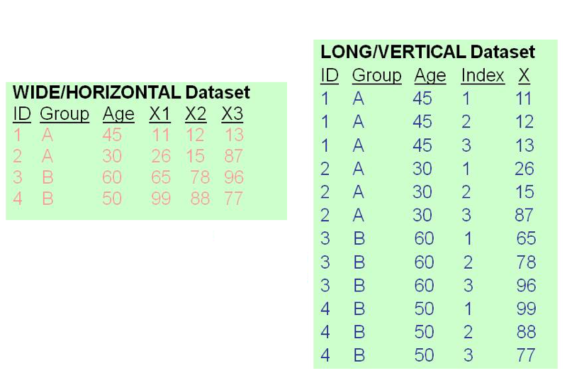
In this example, the wide format of the data has each row representing a single observation. The variables X1, X2 and X3 are what make this “wide”. These are typically variables measured at different time points, but don’t have to be. In the long format, each row represents an observation at a specific index.
A nice feature of Stata’s reshape command is that the syntax to convert from wide-to-long or from long-to-wide are identical, except for desired format (long vs wide).
Convert to long:
reshape long <stub>, i(<ivar>) j(<jvar>)Convert to wide:
reshape wide <stub>, i(<ivar>) j(<jvar>)We need to identify three components, the stub, ivar and jvar.
- “stub”: The stub in wide format is the common prefix of the repeated variables names. In the illustration above,
X1,X2andX3have the common prefix “X”. In the long format, the stub is simply the name of the variable which is repeated. In the illustration above,Xis this variable. Hence the stub isXfor both. - “ivar”: The ivar is the id variable. In the long format, this should be constant across individuals. In both formats above, the id is
ID. - “jvar”: The jvar in long format is the variable that distinguishes which index each repeated measure is from. In the illustration above,
Indexfills this role. In wide format, this does not exist. So when converting from wide to long, you can use any name for the jvar.
Putting this all together together, the two commands to convert between the illustrations above would be:
reshape long X, i(ID) j(Index)
reshape wide X, i(ID) j(Index)
As an example, we’ll use the built-in data set “bplong”
. sysuse bplong, clear
(Fictional blood-pressure data)

. list in 1/5

     +----------------------------------------+
     | patient    sex   agegrp     when    bp |
     |----------------------------------------|
  1. |       1   Male    30-45   Before   143 |
  2. |       1   Male    30-45    After   153 |
  3. |       2   Male    30-45   Before   163 |
  4. |       2   Male    30-45    After   170 |
  5. |       3   Male    30-45   Before   153 |
     +----------------------------------------+
Each patient has two rows representing their before and after measurements. when indicates which time period the measurement occurs in, and bp is the only time-varying variable (both sex and agegrp are constant, presumably the “Before” and “After” occur within a short time period such that neither of those can change). Let’s identify the three components
- “stub”: Since we’re going from long to wide, the “stub” is any time-varying variables, here only
bp. - “ivar”:
patientidentifies individuals. - “jvar”:
whenidentifies time period.
Putting this together,
. reshape wide bp, i(patient) j(when)
(j = 1 2)

Data                               Long   ->   Wide
-----------------------------------------------------------------------------
Number of observations              240   ->   120
Number of variables                   5   ->   5
j variable (2 values)              when   ->   (dropped)
xij variables:
                                     bp   ->   bp1 bp2
-----------------------------------------------------------------------------

. list in 1/5

     +-------------------------------------+
     | patient   bp1   bp2    sex   agegrp |
     |-------------------------------------|
  1. |       1   143   153   Male    30-45 |
  2. |       2   163   170   Male    30-45 |
  3. |       3   153   168   Male    30-45 |
  4. |       4   153   142   Male    30-45 |
  5. |       5   146   141   Male    30-45 |
     +-------------------------------------+
Each row represents a single patient, and bp1 and bp2 represent the before and after measurements.
Let’s generate the command to convert back to long.
- “stub”: “bp” is the stub of
bp1andbp2. - “ivar”:
patientidentifies individuals. - “jvar”: Since the data is currently wide, there is no existing jvar and we can call it whatever we like. For consistency, we’ll call it “when” again.
The command is identical! Just swap wide for long.
. reshape long bp, i(patient) j(when)
(j = 1 2)

Data                               Wide   ->   Long
-----------------------------------------------------------------------------
Number of observations              120   ->   240
Number of variables                   5   ->   5
j variable (2 values)                     ->   when
xij variables:
                                bp1 bp2   ->   bp
-----------------------------------------------------------------------------

. list in 1/5

     +----------------------------------------+
     | patient     when    bp    sex   agegrp |
     |----------------------------------------|
  1. |       1   Before   143   Male    30-45 |
  2. |       1    After   153   Male    30-45 |
  3. |       2   Before   163   Male    30-45 |
  4. |       2    After   170   Male    30-45 |
  5. |       3   Before   153   Male    30-45 |
     +----------------------------------------+
The variables are slightly out of order, but we’ve completely recovered the original data.
After you’ve run a single reshape command, and assuming nothing has changed (you do not want to change stub, ivar or jvar, and the variables in the data are the same), you can convert between wide and long without specifying anything. Try it:
reshape wide
reshape long
Now, notice that when we reshaped the original long data into wide format, the two “bp” variables where bp1 and bp2, not something like bp_before and bp_after. In most cases this is fine (as the common use case for this is repeated measures over time), but not always - what if we wanted to save the “before” and “after” labels? Do note that thankfully Stata saves these labels, so when converting back to long, it restores the “Before” and “After” tags.
If you do want to save the text instead of the count, you need to use strings. We’ll use decode to convert to a string, then use that as the jvar.
. decode when, gen(when2)

. drop when

. rename when2 when

. reshape wide bp, i(patient) j(when) string
(j = After Before)

Data                               Long   ->   Wide
-----------------------------------------------------------------------------
Number of observations              240   ->   120
Number of variables                   5   ->   5
j variable (2 values)              when   ->   (dropped)
xij variables:
                                     bp   ->   bpAfter bpBefore
-----------------------------------------------------------------------------

. list in 1/5

     +----------------------------------------------+
     | patient   bpAfter   bpBefore    sex   agegrp |
     |----------------------------------------------|
  1. |       1       153        143   Male    30-45 |
  2. |       2       170        163   Male    30-45 |
  3. |       3       168        153   Male    30-45 |
  4. |       4       142        153   Male    30-45 |
  5. |       5       141        146   Male    30-45 |
     +----------------------------------------------+
Note the string option. When converting back to long, you’ll need to encode the string to get it back to numeric.
. reshape long
(j = After Before)

Data                               Wide   ->   Long
-----------------------------------------------------------------------------
Number of observations              120   ->   240
Number of variables                   5   ->   5
j variable (2 values)                     ->   when
xij variables:
                       bpAfter bpBefore   ->   bp
-----------------------------------------------------------------------------

. desc when

Variable      Storage   Display    Value
    name         type    format    label      Variable label
-------------------------------------------------------------------------------
when            str6    %9s                   Status

. encode when, gen(when2)

. drop when

. rename when2 when

. desc when

Variable      Storage   Display    Value
    name         type    format    label      Variable label
-------------------------------------------------------------------------------
when            long    %8.0g      when2      Status
A few notes:
If you have wide data and some individuals are missing some repeated measures, when converting to tall, they will still have a row with a blank value. You can easily drop it:
reshape long
drop if <varname> == .
Converting back to wide will re-enter those missing values;
reshapedoes not care if the long data is “complete”.More than one stub can be entered if you have more than one repeated measurement. For example, if the variables were {“id”, “x1”, “x2”, “y1”, “y2”}, you could enter
reshape long x y, i(id) j(index)Note that they technically don’t have to have the same indices (e.g. you could have “x1”, “x2”, “y3”, “y4”) although that would create a weird result where each row of index 1 or 2 is missing
yand each row of index 3 or 4 is missingx.If you have wide data and many time-varying variables, there is no shorthand for entering all the stubs. For large data, this is extremely frustrating. I’d recommend using
describe, simpleto get a list of all variable names, then using find & replace to remove the indices. If you know a better way, let me know!
If you want log with a different base, you can use the transformation that dividing by
log(b)is equivalent to usingbas a base. In other words, if you need log base 10, usegen newvar = log(oldvar)/log(10).↩︎Technically and mathematically they can take on any two values, but your life will be easier if you stick with the 0/1 convention.↩︎
This is true of most statistical software in fact.↩︎
We’ll see some exceptions to this in the programming section.↩︎
egenis not a short command for “egenerate”; the full command name is simply “egen”.↩︎generatehas a few features we do not discuss whichreplacedoes not support. Namely,generatecan set the type manually (instead of letting Stata choose the best type automatically), andgeneratecan place the new variable as desired rather than usingorder. Clearly, neither of these features are needed forreplace.↩︎Note that this is not a statistical claim, we would have to do a two-sample t-test to make any statistical claim.↩︎
I’m explcitly writing the quotations here as otherwise it would just look missing. The quotations aren’t part of the saved string.↩︎
If you are sharp-eyed, you may have noticed that the original
mpgwas an “int” whereas the final one is a “byte”. If we had calledcompresson the original data, it would have done that type conversion anyways - so we’re ok!↩︎